Assessing the non-uniform vulnerability of vegetation productivity and canopy structure under drought stress
-
摘要:
频繁的干旱事件已对植被正常生长与生态系统稳定构成威胁。为解析干旱对植被影响的复杂性,该研究基于Copula模型,利用归一化植被指数、总初级生产力和标准化降水蒸散发指数,构建了气象干旱胁迫下植被生产力与冠层结构损失的条件概率模型,并运用偏最小二乘路径模型,探讨了植被对干旱响应的驱动因子。结果表明,1982—2018年长江流域植被生产力、冠层结构对气象干旱的滞后响应在时间维和空间维呈现出非一致性特征。时间上,植被生产力对气象干旱的响应时间较冠层结构更长;空间上,汉江流域和长江中下游干流区植被生产力易损性高,而金沙江流域和长江干流区间冠层结构易损性高。不同类型植被的易损性不同,水田和常绿阔叶林的生产力损失概率较高,分别为21.05%、17.26%,草地和常绿针叶林的冠层结构损失概率更大,分别为36.35%、35.73%。此外,植被生产力与冠层结构的关键环境影响因子不同,前者主要受控于冠层结构和土壤水分,后者则对海拔和气候因子更为敏感。研究成果有助于深入了解干旱对植被的影响,进而为生态系统管理与保护提供重要的科学依据。
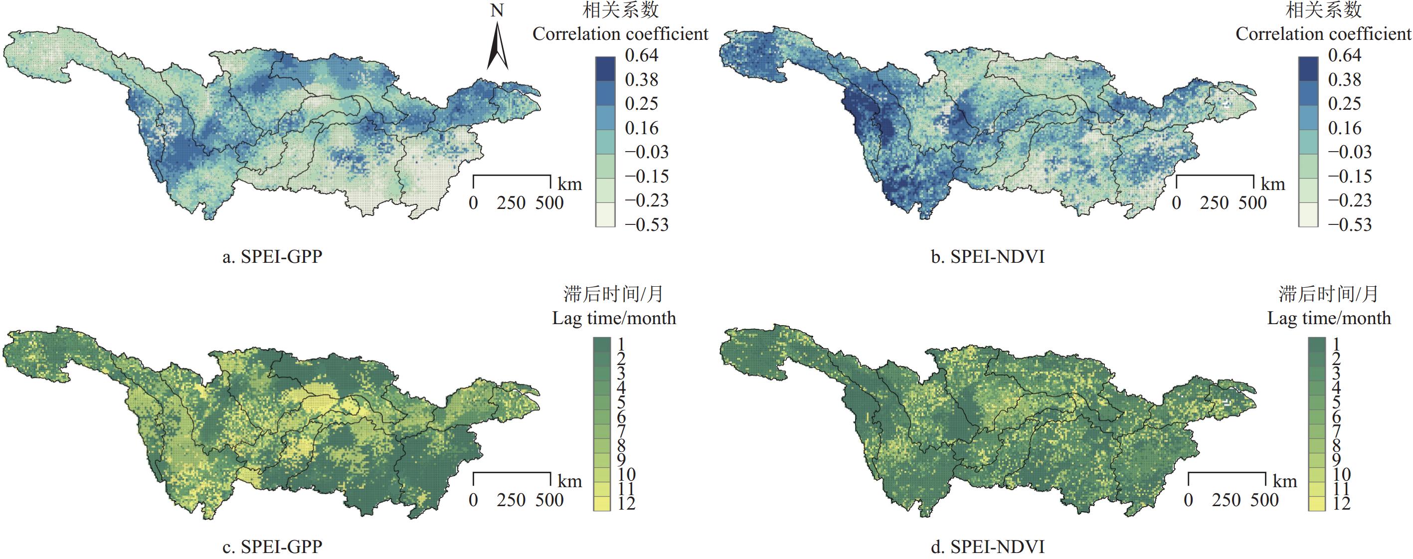
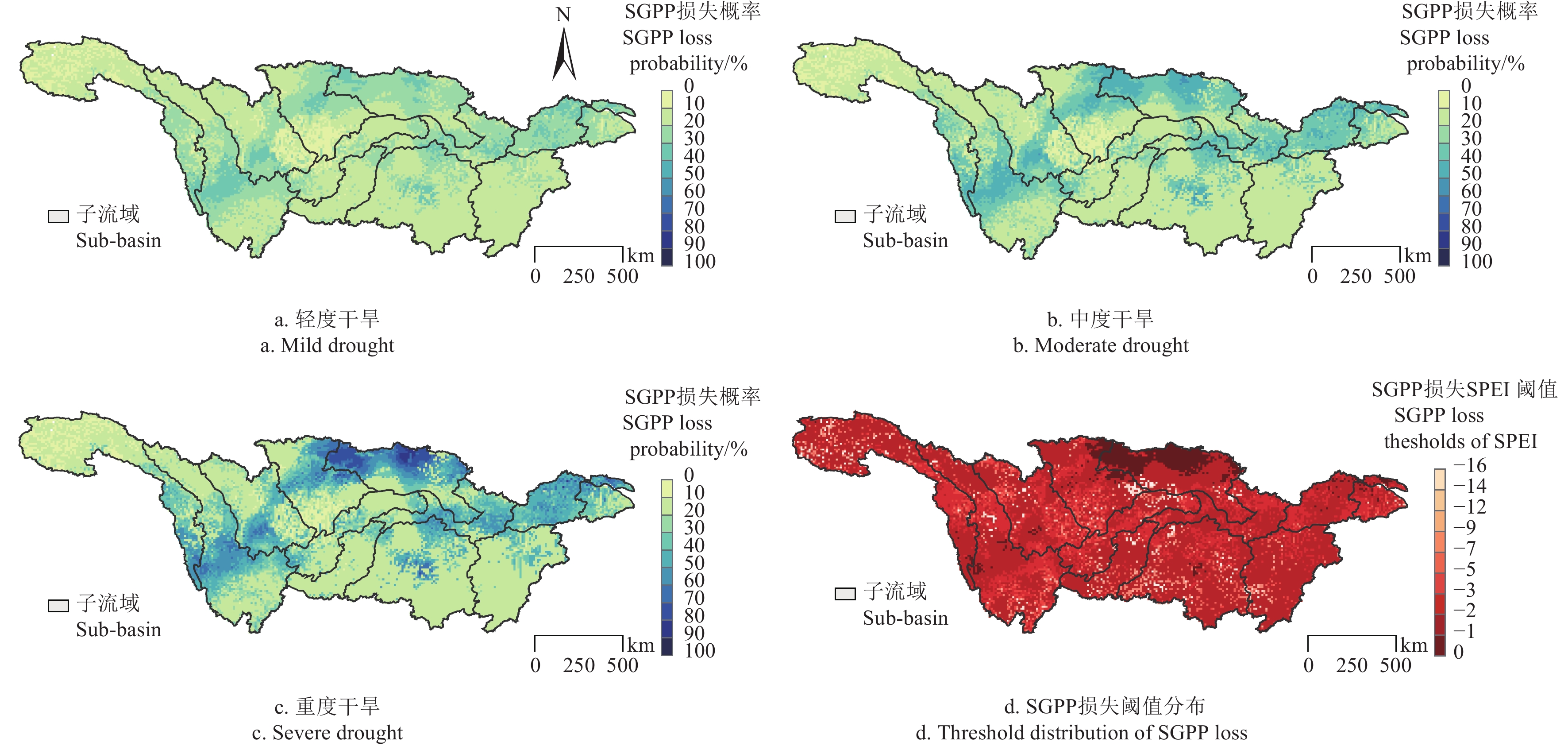
Abstract:Frequent and severe drought events have posed the serious threat to vegetation growth and ecosystem stability. The underlying dynamics of vegetation response to droughts can be expected to predict and mitigate the impacts of these environmental stresses on ecosystems. However, a single ecological index cannot fully meet the requirements of the vegetation responses to droughts. In this study, a robust conditional probability model was constructed to combine the normalized difference vegetation index (NDVI), gross primary productivity (GPP), and the standardized precipitation and evapotranspiration index (SPEI). The Copula framework was designed to clarify the relationships between meteorological drought stress and the probabilities of vegetation productivity and canopy structure loss. Additionally, a systematic investigation was also made to explore the interactions between different vegetation growth statuses and environmental factors, as well as the driving forces behind drought trigger thresholds using partial least squares path modeling (PLS-PM). A case study was also carried out in the Yangtze River Basin (YRB) from 1982 to 2018. The temporal and spatial disparities were observed in the vegetation productivity and canopy structure response to the meteorological droughts. The results indicate that: 1) The proportion of areas where vegetation productivity and canopy structure in the YRB are positively correlated with SPEI is 50.61% and 63.04%, respectively.. Notably, the canopy structure exhibited a closer association with the SPEI, compared with the vegetation productivity. There was a shorter response time to the meteorological drought stress. The canopy structure shared the higher vulnerability under drought duress, compared with the vegetation productivity. 2) Spatially, the high vulnerability was found in regions, such as the Hanjiang Basin and the middle and lower reaches of the Yangtze River, in terms of vegetation productivity. While the increasing susceptibility of canopy structure was displayed in the Jinsha River Basin and the mainstream of the Yangtze River. 3) The average probabilities of loss were 20.04%, 23.63%, and 28.99%, respectively, for vegetation productivity under mild, moderate, and severe drought stress. The heightened vulnerability was predominantly concentrated in the Hanjiang Basin and the middle and lower reaches of the Yangtze River. Canopy structures shared the average probabilities of loss of 23.26%, 24.77%, and 26.86% under similar drought stress levels. Among them, the regions of elevated vulnerability were located primarily in the Jinsha River Basin. 4) There were starkly pronounced disparities of vulnerability among various vegetation types over the basin. Irrigated cropland and evergreen broadleaf forests showed higher-than-average probabilities of productivity loss (21.05% and 17.26%, respectively). While the grasslands and evergreen needleleaf forests demonstrated elevated probabilities of canopy structure loss (36.35% and 35.73%, respectively). Furthermore, the wetter regions exhibited higher average probabilities of vegetation productivity loss under varying intensities of drought stress. While the drier regions showed the heightened average probabilities of canopy structure loss. 5) Canopy structure was more susceptible to external disturbances. While the vegetation productivity was dominated by the soil moisture and its own canopy structure. There was a complex interplay between vegetation responses to drought and environmental factors in the YRB. The findings can provide invaluable insights for the effective management and conservation of ecosystems against droughts.
-
0. 引 言
猕猴桃是陕西省的重要地标产品,种植面积和产量均居陕西前列。在规模化发展中,水分管理是关键“因素”之一[1-3]。有效的水分管理在果实膨大期起到关键作用。猕猴桃对水分需求较高,土壤水分不足会严重影响果实生长和单果质量,导致产量与品质下降,削弱市场竞争力[4-5]。传统的土壤水分采集手段主要有直接取样法、水分传感器法和重量法[6],不仅数据采集效率较低,且对土壤有一定程度的破坏,从而无法大规模的对果园进行有效的水分管理,因此需要找到一种连续、准确、灵活的土壤水分监测系统。
近年来,大规模的土壤水分监测主要是通过无人机遥感和卫星遥感获取微波、热红外和光学遥感数据结合机器学习去反演土壤水分[7]。其中微波遥感技术在土壤水分监测领域取得了显著进展,特别是合成孔径雷达(synthetic aperture radar,SAR)技术的发展,使其在探测一定深度的根域土壤水分方面展现出巨大的潜力,但微波遥感常搭载卫星无法高精度且连续的监测特定区域的土壤水分[8]。相比之下,无人机光学遥感技术因其高效、便捷、覆盖范围广等特点已广泛应用果园的土壤水分监测。靳亚红等[9]利用无人机多光谱遥感数据,通过皮尔逊相关系数和XGBoost模型反演玉米和小麦的土壤含水率。喷灌条件下的最优光谱窗口较畦灌小,玉米灌浆期的R2分别为0.80(喷灌)和0.83(畦灌),RMSE为1.27%和0.98%;小麦苗期的R2为0.76(喷灌)和0.79(畦灌),RMSE分别为1.68%和0.85%。该研究为基于无人机遥感的土壤水分监测提供了有效的方法。在果园方面,DENG等[10]通过多层感知器模型结合冠层植被指数评估猕猴桃果园的土壤水分,R2为
0.744; ZHU等[11]通过利用无人机多光谱影像特征与集成学习方法,结合最优波段组合算法,评估了猕猴桃冠层反射率和植被覆盖度特征对根域土壤水分的敏感性。这些为果园中精确的土壤水分监测提供了一种可行的技术路径。同时深度学习的模型改进也成为研究的关键方向。潘时佳等[12]使用无人机搭载多光谱相机获取的数据,通过MLP网络和CVCRNet模型,探索了植被指数与土壤含水率的关系。综上所示,尽管当前利用无人机多光谱成像技术应用在土壤水分监测中已经取得了显著进展[13-15],但大多数现有方法主要集中在图像信息的处理和模型的改进,然而土壤水分监测是一种动态变化,则需要通过输入信息的时间序列来动态反演果园土壤水分的变化。该研究针对目前存在的问题,特别是在时序问题的处理和土壤水分监测的连续性方面的不足,以眉县猕猴桃果实膨大期为研究对象,提出了一种基于无人机遥感技术与时序模型结合的猕猴桃根域土壤水分时序反演方法,获取根域土壤水分的动态变化情况,同时可以为其他的果园作物的水分管理提供一定的参考。
1. 材料和方法
1.1 试验区域
试验地点位于陕西省宝鸡市眉县西北农林科技大学猕猴桃农业气象科技小院,北纬107°59′,东经34°7′,海拔 643.22 m。四季分明,夏季炎热,冬季寒冷,多年平均降水量为 609.5 mm,年均日照时数为
2015.2 h。猕猴桃果树每年6月初进入果实生长期,冠层生长完全覆盖地面,对水分和养料的需求显著增加。区域总面积约6000 m2 ,试验区域面积约 300 m2 ,品种为徐香猕猴桃,共 4 行 6 列,株距约 3 m,行距约 4 m,分布如图1所示,从早春萌芽前1个月开始到萌芽后约2个月进行剪枝管理,同时果园内架设钢丝以供猕猴桃藤蔓生长缠绕。试验于 2023 年 6 月 7 日开始, 60 d连续监测。为了保证试验的一致性,测量时间为 11:30—12:00 ,试验期间根据土壤表面视觉观察情况进行灌溉。每棵猕猴桃果树的每日遥感数据和土壤含水率为一组基础数据,共有基础数据
1440 组,将原始数据集随机划分,其中 80% 的数据作为训练集,20% 的数据作为测试集。1.2 地面土壤水分数据收集
土壤水分测量采用土壤温度水分变送器(485型),其原理利用传感器测量土壤中的温度和水分,通过数据转换器将测量结果以模拟信号(如4~20 mA)传输至记录仪。土壤含水率的计算式:
土壤含水率(%)=(土壤水分体积土壤体积)×100% (1) 首先,选择尽量靠近待测猕猴桃主干距离 1 m 内且深度0.4 m处埋置监测仪探针,该区域位于猕猴桃果树根域深度的水分活跃层(0.2~0.8 m),该层受灌溉和降雨影响显著,且深度大于0.2 m,受大气环境影响较小。每棵猕猴桃果树埋置一根探针,该相对位置如图1所示。每次测量重复3次,去除异常值后取平均值,作为被测果树的根域土壤水分。试验期间各组平均土壤含水率范围为 22.2%~42.5%。分别在6月17日、6月28日、7月03日、7月14日分别有降水出现,实际根域土壤水分变化情况如图2(选择试验区域内5棵猕猴桃根域土壤含水率做为代表)。
1.3 无人机遥感数据采集与预处理
1.3.1 遥感数据采集
遥感图像的采集采用搭载RTK模块的DJI Mavic 3多光谱版无人机,共集成 4 个多光谱镜头,分别对应绿波段(560±16)nm、红波段(650±16)nm、红边波段(730±16)nm、近红外波段(860±26)nm,为确保区域图像边缘的完整性,航拍区域覆盖整个试验区域适当扩大。每次飞行持续 276 s ,覆盖面积为 964 m2 ,并与地面土壤水分观测同步进行。飞行高度 15 m ,巡航速度 5 m/s ,航拍旁向重叠率和航向重叠率均为 80% ,拍摄方向为竖直向下。在无阴影遮挡的位置放置MAPIR多光谱校准标定板,以确保数据的准确性。获得的原始多光谱图像通过Pix4D Mapper进行几何校正和辐射校正,生成试验地多光谱正射影像。
1.3.2 光谱反射率提取
生成多光谱正射影像以后需要对单株猕猴桃多光谱感兴趣区域范围进行平均光谱反射率提取,但由于猕猴桃果园的冠层信息分布与大田作物存在显著差异。其冠层结构复杂,冠层信息与根域土壤水分在空间上无法直接对应。对于小麦、玉米等大田作物(图3a)其冠层数据与根域土壤的位置几乎垂直对应,而猕猴桃果树的冠层覆盖范围较大,且存在相互交叉现象(图3b),传统的采样方式难以准确获取目标区域的植被指数,导致与根域土壤水分的相关性降低。
![]() 图 3 冠层与土壤信息的空间映射关系Figure 3. Spatial mapping relationship between canopy and soil information
图 3 冠层与土壤信息的空间映射关系Figure 3. Spatial mapping relationship between canopy and soil information为了确定单棵猕猴桃树的冠层分布范围并解决冠层相互交叉的问题,冠层范围采样法融合了冬季骨架信息与夏季冠层叶片信息,对猕猴桃冠层进行多级综合分析,从而提取单株植株的冠层范围。骨架预测和图像合并技术,即使在冠层密集且存在交叉的果园中,也能有效地分离出单个冠层[16]。最后,通过对传统矩形采样法(图4a)和冠层范围采样法(图4b)进行对比,验证了两种方法在提取平均光谱反射率计算出的植被指数与根域土壤水分相关性方面的效果差异,从而选取更优的采样方法去提取四波段平均光谱反射率(图4)。
1.3.3 植被指数(vegetation index,VI)特征提取
在提取单株猕猴桃的四波段平均反射率以后,为得到猕猴桃根域土壤含水率与遥感数据之间的确切关系,依据表1中的计算式初步选择20种对土壤水分较为敏感的植被指数[17-23]作为猕猴桃根域土壤水分模型的原始数据。
表 1 植被指数计算式Table 1. Vegetation index formula植被指数Vegetation index(VI) 计算式Formula 参考文献 Reference 绿色指数Green index(GI) ρGRE/ρGREρREDρRED [17] 修改型土壤调整植被指数Modified soil adjusted vegetation index(MSAVI) 0.5×(2×ρNIR+1−√(2×ρNIR+1)2−8(ρNIR−ρRED)) [17] 绿度归一化植被指数Green normalized difference vegetation index(gNDVI) (ρNIR−ρGRE)/(ρNIR−ρGRE)(ρNIR+ρGRE)(ρNIR+ρGRE) [18] 归一化植被指数Normalized difference vegetation index(NDVI) (ρNIR−ρRED)/(ρNIR−ρRED)(ρNIR+ρRED)(ρNIR+ρRED) [18] 优化土壤调节植被指数Optimized soil adjusted vegetation index(OSAVI) (ρNIR−ρRED)/(ρNIR−ρRED)(ρNIR+ρRED+0.5)(ρNIR+ρRED+0.5) [18] 重归一化植被指数Renormalized difference vegetation index(RDVI) (ρNIR−ρGRE)/(ρNIR−ρGRE)(√ρNIR+ρGRE)(√ρNIR+ρGRE) [18] 土壤调整植被指数Soil adjusted vegetation index(SAVI) (ρNIR−ρRED)/(ρNIR−ρRED)(ρNIR+ρRED+L)(ρNIR+ρRED+L)×(1+L)* [19] 简单比值指数Simple ratio index(SR) ρNIR/ρNIRρREDρRED [19] 绿色叶绿素植被指数Green chlorophyll vegetation index(GCVI) ρNIR/ρGRE−1 [20] 植物衰老反射指数Plant senescence reflection index(PSRI) (ρRED−ρGRE)/ρREG [20] 红边归一化差异植被指数Red-edge normalized difference vegetation index(NDVIre) (ρNIR−ρREG)/(ρNIR+ρREG) [21] 修正型红边简单比值指数Modified red-edge simpleratio index(MSRre) (ρNIR/ρREG−1)/(√ρNIR/ρREG+1)(√ρNIR/ρREG+1) [21] 红边叶绿素指数Red-edge chlorophyll index(CIre) ρNIR/ρREG−1 [21] 红边简单比率指数Red-edge simple ratio index(SRre) ρNIR/ρREG [21] 双波段增强植被指数Two-band enhanced vegetation index(EVI2) 2.5×(ρNIR−ρRED)/2.5×(ρNIR−ρRED)(ρNIR+2.4ρRED+1)(ρNIR+2.4ρRED+1) [22] 陆地叶绿素指数MERIS terrestrial chlorophyll index(MTCI) (ρNIR−ρREG)/(ρNIR−ρREG)(ρREG+ρRED)(ρREG+ρRED) [22] 归一化差值水体指数Normalized difference water index(NDWI) (ρGRE−ρNIR)/(ρGRE−ρNIR)(ρGRE+ρNIR)(ρGRE+ρNIR) [23] 全球环境监测指数Global environment monitoring index(GEMI) eat×(1−0.25×eat)−(ρRED−0.125)/−(ρRED−0.125)(1−ρRED)(1−ρRED)eat=(2×(ρ2NIR−ρ2RED)+1.5×ρNIR+0.5ρRED)/+1.5×ρNIR+0.5ρRED)(ρNIR+ρRED+0.5)(ρNIR+ρRED+0.5) [23] 红边三角植被指数Red-edge triangular vegetation index(RTVICore) 100×(ρNIR−ρREG)−10×(ρNIR−ρGRE) [24] 修正型三角植被指数Modified triangular vegetation index(MTVI2) 1.5×(1.2×(ρNIR−ρGRE)−2.5×(ρRED−ρGRE))×√(2×ρNIR+1)2−(6×ρNIR−5√ρRED)−0.5 [24] 注:ρGRE为绿波段平均反射率;ρRED为红波段平均反射率;ρREG为红边波段平均反射率;ρNIR为近红外波段平均反射率。L为土壤亮度校正因子,根据覆盖量此处取L=0.90。 eat为中间变量,通过近红外和红光波段的值按照特定公式计算得出。
Note: ρGRE is the average reflectance of green band; ρRED is the average reflectance of the red band; ρREG is the average reflectance of the red-edged band; ρNIR is the average reflectance of near infrared band. L is the correction factor for soil brightness, L=0.90 is taken here according to the coverage amount. eat is the intermediate variable, which is calculated by the values of near-infrared and red wavelengths according to a specific formula.1.3.4 植被指数(VI)特征筛选
为筛选出与根域土壤含水率具有显著相关性的植被指数特征,并有效提升模型的预测性能和稳定性,同时减少过拟合风险,综合运用了Pearson相关系数和Spearman秩相关系数进行特征筛选[24]。在Pearson和Spearman分析中,筛选标准设定为P ≤ 0.05,表示相关性具有统计显著性。具体而言,Pearson相关系数用于评估植被指数与根域土壤水分之间的线性关系,而Spearman秩相关系数则用于检测非线性关系。通过同时应用这两种方法,能够确保所选特征在不同类型的关系下均具有显著统计学意义,从而减少依赖单一方法可能带来的偏误。各特征的相关性系数绝对值越大,表明该特征对模型的重要性越高,有助于提高模型的稳定性与预测准确性。
1.4 模型构建
1.4.1 基于非时序网络的根域土壤含水率反演模型
为对比非时序网络与时序网络的性能差异,首先引入传统的前馈神经网络(feedforward neural network,FFNN)进行反演。根据第 1.3.4 节筛选出植被指数作为模型输入,以对应的根域土壤含水率为网络输出,网络基本结构如图5 所示。
![]() 图 5 FFNN 非时序网络结构示意图注:其中VI1~VIx为各输入植被指数 Note: VI1~VIx refers to the input vegetation indexFigure 5. Structure of FFNN(feed forward neural network) non-temporal network structure
图 5 FFNN 非时序网络结构示意图注:其中VI1~VIx为各输入植被指数 Note: VI1~VIx refers to the input vegetation indexFigure 5. Structure of FFNN(feed forward neural network) non-temporal network structure为了获得最优模型,确保模型的损失函数值下降到较低水平并收敛,设定训练批次(batch size)为 10,选择 Adam 优化器,初始学习率设置为 0.001,学习率衰减范围设置为 0.9~0.999。
选取均方误差(mean square error,MSE)作为损失函数,其计算式:
MSE=N∑i(yturei−yprei)2N (2) 式中yprei表示样本i的估测值;yturei表示样本i的真实值,N表示变量的个数。
使用不同参数选择下的最优迭代结果,对训练集和测试集样本的根域土壤含水率估算结果进行对比,从而确定建立的非时序FFNN网络结构网络类型为全连接网络,第一层节点数50,中间层结构(100,5),输出层节点数为1,激活函数为ReLu。
1.4.2 基于时序网络的根域土壤含水率反演模型
为更好地捕捉猕猴桃果园中土壤水分的时序变化规律,本节在FFNN网络结构基础上进行改进,将其输入层替换为LSTM(long short-term memory)层或BiLSTM(bidirectional long short-term memory)层[17-23]。LSTM和BiLSTM本身是专为处理时间序列数据而设计的模型,能够有效地捕捉土壤水分在时间维度上的动态变化。LSTM层能够记住并传递长时间间隔内的重要信息,而BiLSTM层则通过同时从过去和未来的时间点提取信息,进一步提升了模型的时序捕捉能力,该节为了避免过拟合在原基础上中增加了多个Dropout层,以0.5的概率随机舍弃部分全连接层参数,建立的LSTM网络(图6a)和BiLSTM网络(图6b)结构。
对于时序反演模型主要需要定义两个超参数:历史关注步长(input_steps)和预测序列长度(predict_steps),其中,input_steps为模型输入的数据天数;predict_steps 为模型需要预测的时间步数,input_steps设置为3~7,predict_steps 设置为 1。
利用滑动窗口方法在时序数据上构建样本,如图7 所示。具体过程如下,以 input_steps 为 3作为模型输入,以当日的根域土壤含水率为输出为例:
构建第一个样本:从第一个时间点开始,取前 3 d的植被指数作为输入特征,第三天的根域土壤含水率作为目标值:features = [(V1),(V2),(V3)],target = (D3)滑动窗口移动:features = [(V2),(V3),(V4)], target = (D4)最终获得 58 组数据。
1.5 训练平台与精度评估
该试验在 Windows 10 专业版操作系统(Microsoft)上进行。系统硬件配置包括 NVIDIA GeForce RTX
3060 GPU、AMD Ryzen 7 5800H 处理器以及 32GB DDR4 内存。软件环境方面,使用 Anaconda3.0 搭建 TensorFlow 框架,并在 Python 3.8.13 版本下进行网络的构建与训练。为了评估模型的预测精度,采用决定系数和均方根误差作为评价指标,其计算式:R2=∑(ypre−ˉy)2∑(ytrue−ˉy)2 (3) RMSE=√∑(ypre−ytrue)2N (4) 式中ytrue表示真实值;ypre表示估测值,ˉy表示全部真实值的均值。
2. 结果与分析
2.1 不同光谱反射率采样法结果对比
为了具体分析不同采样法的显著性,将分析结果汇总得到表2,在使用Pearson和Spearman相关系数进行评估时,传统矩形采样法有8种植被指数表现出显著性,而冠层范围采样法则有9种植被指数具有显著性,在这些植被指数中,冠层范围采样法与土壤含水率的相关性较高,因此该研究冠层采样法进行非时序模型构建。选择9种(SR、NDVI、GI、OSAVI、MSAVI、SAVI、PSRI、EVI2和MTCI)植被指数作为非时序模型的原始输入。此外,为了减少试验结果的偶然性,还将在9种的基础上额外选取6种(GCVI、GEMI、MTVI2、gNDVI、RDVI和NDWI)仅在线性相关性分析中具有显著性的植被指数作为对比输入(方案2),从而确定非时序与时序模型的最终输入。
表 2 基于不同采样方法的20种植被指数Pearson与Spearman相关性分析表Table 2. Pearson and Spearman correlation analysis table of 20 planting indices based on different sampling methods植被指数 传统采样法
Traditional sampling method冠层采样法
Canopy sampling methodVegetation index Pearson Spearman Pearson Spearman SR 0.29* 0.19* 0.33* 0.20* SRre 0.18* −0.05 0.12 0.13 NDVI 0.24* 0.19* 0.30* 0.20* gNDVI 0.11 0.08 0.21* 0.12 NDVIre 0.16* −0.05 0.092 0.13 CIg 0.17* 0.08 0.25* 0.12 Clre 0.18* −0.05 0.12 0.13 GI 0.29* 0.26* 0.26* 0.16* OSAVI 0.24* 0.18* 0.30* 0.20* RDVI 0.14* 0.04 0.19* 0.10 MSAVI 0.22* 0.19* 0.29* 0.20* SAVI 0.24* 0.18* 0.30* 0.20* PSRI −0.21* −0.25* −0.17* −0.15* MSRre 0.17* −0.05 0.12 0.13 EVI2 0.26* 0.18* 0.31* 0.20* MTCI 0.20* −0.01 0.17* 0.16* GEMI −0.19* −0.06 −0.20* −0.10 MTVI2 0.21* 0.04 0.19* 0.14 NDWI −0.11 −0.08 −0.21* −0.12 RTVICore 0.17* 0.07 0.12 0.12 注:*表示在P≤ 0.05时,该植被指数具有显著性。
Note: * indicates that the vegetation index is significant when P≤0.05.2.2 非时序网络反演结果
首先,分别使用FFNN网络对9种植被指数输入和15种植被指数输入进行非时序模型构建,筛选出在测试集样本中RMSE最小的迭代结果作为最终训练结果(见表3)。在训练集上,使用15种植被指数时,模型的R2为0.384,RMSE为3.15%;而使用9种植被指数时,R2为0.432,RMSE为3.56%。该结果表明9种植被指数数量作为输入的反演效果更加稳定,故该研究选择9种植被指数作为时序与非时序模型的最终输入。
表 3 不同数量植被指数非时序网络根域土壤水分反演精度Table 3. Precision of root soil moisture retrieval using non- temporal networks with different vegetation index numbers植被指数数量
Vegetation index numbersR2 RMSE/% 训练集
Training set测试集
Test set训练集
Training set测试集
Test set9 0.432 0.269 2.99 3.56 15 0.384 0.254 3.15 3.61 2.3 时序网络反演结果
为验证时间序列信息对根域土壤含水率反演的影响,该研究构建了以多日植被指数为输入的数据集,并结合LSTM与BiLSTM进行建模。历史关注步长设置为3~7天,分别进行迭代训练,结果如表4所示。
表 4 不同历史关注步长下时序网络最佳迭代次数Table 4. Optimal iteration times for time-series networks under different history focuses on step size历史关注步长History focuses on step size LSTM BiLSTM 3 470 590 4 505 610 5 595 590 6 300 570 7 320 410 在训练集和测试集(表5)上,对比不同历史关注步长对应的测试结果发现,LSTM 网络和BiLSTM 网络均在历史关注步长为 5 天时效果最佳。
表 5 不同历史关注步长下时序网络的反演精度Table 5. Inversion accuracy of temporal networks with different history focuses on step size网络
Network历史关注步长
History focuses on step sizeR2 RMSE/% 训练集
Training set测试集
Test set训练集
Training set测试集
Test setLSTM 3 0.473 0.413 2.88 2.97 4 0.661 0.402 2.35 2.80 5 0.842 0.548 1.59 2.68 6 0.609 0.538 2.46 2.80 7 0.722 0.515 2.12 2.81 BiLSTM 3 0.552 0.537 2.66 2.67 4 0.676 0.488 2.33 2.65 5 0.815 0.624 1.74 2.45 6 0.797 0.587 1.82 2.70 7 0.775 0.485 1.91 2.93 在最优历史关注步长下,对LSTM和BiLSTM网络的模型表现(图8)。图8a显示,LSTM网络在迭代次数小于300时,训练集和测试集的损失函数值显著下降,模型逐渐收敛;相比之下,图8b表明,BiLSTM网络的损失函数值下降趋势更明显,在360至530次迭代间达到最佳效果,且测试集损失函数值更低,模型收敛效果更佳。
![]() 图 8 不同时序网络训练过程中损失函数值变化Figure 8. The loss function value changes during the training of different time series network
图 8 不同时序网络训练过程中损失函数值变化Figure 8. The loss function value changes during the training of different time series network结合散点图(图9)分析,在训练集上,LSTM的拟合效果略优于BiLSTM,R2为0.842,RMSE为1.59%;BiLSTM 的R2为 0.815,RMSE为1.74%。然而,在测试集上,BiLSTM 网络表现出更好的泛化能力,R2为0.624,RMSE为 2.45%,优于LSTM网络(R2为 0.548,RMSE为 2.68%)。
![]() 图 9 时序网络的根域土壤含水率反演结果Figure 9. Inversion results of soil moisture using temporal network
图 9 时序网络的根域土壤含水率反演结果Figure 9. Inversion results of soil moisture using temporal network2.4 基于不同模型反演效果分析
为了体现不同时间尺度下的时序与非时序反演效果,该研究构建传统前馈神经网络(FFNN)、长短期记忆网络(LSTM)和双向长短期记忆网络(BiLSTM)在最优历史关注步长的反演结果对比,结果如表6所示。
表 6 不同方法对于根域土壤含水率的反演结果Table 6. Inversion results of soil moisture content in root domain by different methods网络
Network历史关注步长
History focuses
on step sizeR2 RMSE/% 训练集
Training set测试集
Test set训练集
Training set测试集
Test setFFNN 5 0.650 0.528 2.40 2.78 LSTM 5 0.842 0.548 1.59 2.68 BiLSTM 5 0.815 0.624 1.74 2.45 结合上表,时序网络模型在测试集上的拟合精度均高于非时序网络模型,具体表现为:
1)FFNN模型:由于模型无法吸收时间序列信息,FFNN模型在测试集上的R2值仅为0.528,RMSE值为2.78%,明显逊色于LSTM和BiLSTM模型。这主要归因于FFNN模型无法有效利用长时间段内的历史信息,限制了其反演精度。
2)LSTM模型:在最优历史关注步长时,测试集上的R2值为0.548,RMSE值为2.68%。这表明LSTM模型能够有效捕捉土壤水分变化的时间序列特征,具有较高的预测准确性。
3)BiLSTM模型:在相同步长下,测试集上的R2值为0.624,RMSE值为2.45%。尽管BiLSTM模型在某些情况下R2值略低于LSTM模型,但其在测试集上的表现更为优异,显示出在处理复杂时间序列数据时具有更强的鲁棒性和泛化能力。
3. 结 论
该研究提出以猕猴桃根域土壤水分为研究对象,通过Pearson与Spearman相关性法筛选植被指数得到最优指标组合,结合传统前馈神经网络(FFNN)、长短期记忆网络(LSTM)和双向长短期记忆网络(BiLSTM)构建猕猴桃果园的根域土壤水分反演模型,并通过采集田间数据证明其可靠性,获得主要结论如下:
1)冠层范围采样法在植被指数与根域土壤水分的线性与非线性相关性上优于传统矩形采样法,能够选择更多显著性相关的植被指数,从而提高模型反演精度。
2)在不同的历史关注步长下,时序网络(LSTM和BiLSTM)相比传统FFNN模型表现出显著的优势。特别是BiLSTM模型,具有更强的泛化能力,在测试集上R2为0.624,RMSE为2.45%,优于LSTM。证明了时序网络能够有效捕捉土壤水分变化的时间序列特征。
-
![]()
图 1 长江流域海拔、子流域分区及土地覆盖类型图
Figure 1. Elevation, sub-basin, and land cover type map of the Yangtze River Basin
![]()
图 2 1982−2018年植被指数与SPEI的最大相关系数及其响应滞后时间分布
注:+ 显著性P<0.05。Note: + indicates significant P<0.05.
Figure 2. Maximum correlation coefficient and response lag time between vegetation indices and SPEI from 1982 to 2018
![]()
图 3 长江流域不同干旱强度下标准化总初级生产力损失概率及干旱触发阈值分布
Figure 3. Probability of standardized gross primary production(SGPP) loss under different drought intensities and distribution of drought trigger thresholds in the Yangtze River Basin
![]()
图 4 长江流域不同干旱强度下标准化归一化植被指数损失概率及干旱触发阈值分布
Figure 4. Probability of standardized normalized difference vegetation index(SNDVI) loss under different drought intensities and distribution of drought trigger thresholds in the Yangtze River Basin
![]()
图 5 不同流域分区、不同干旱强度下的SGPP与SNDVI损失概率分布
Figure 5. Probability of SGPP and SNDVI loss under different watershed delineations and varying drought intensity
![]()
图 6 环境因子主成分分析图
注:DEM,海拔;Temp,气温;VPD,饱和水汽压差;SM,土壤水分;Soiltype,土壤类型。
Figure 6. Principal component analysis (PCA) plot of environmental factors
Note: DEM, elevation; Temp, temperature; VPD, vapor pressure defict; SM, soil moisture; Soiltype, soil type.
![]()
图 7 干旱触发阈值与环境因子的交互作用路径
注:箭头上的数据为标准化路径系数;*和**分别表示P<0.05和P<0.01;R2表示因变量解释的方差比例。
Figure 7. Interaction pathways of the environmental factors and drought index thresholds
Note: The data on the arrow is the standardized path coefficient; * and ** mean P<0.05 and P<0.01 level, respectively; R2 indicates the proportion of variance explained by each dependent variable.
表 1 不同干旱强度胁迫下的植被损失概率及干旱触发阈值
Table 1 Probability of vegetation loss under different drought intensity stresses and drought index threshold
指数
Index植被类型
Vegetation types触发阈值
Drought trigger thresholds植被损失概率
Vegetation loss probability/%轻度干旱
Mild drought中度干旱
Moderate drought重度干旱
Severe droughtSGPP RCA −3.44 12.87 13.58 14.55 ICA −3.39 18.38 20.77 23.98 EBF −3.34 15.56 17.09 19.12 DBF −4.32 12.64 13.23 14.09 ENF −4.04 11.46 11.74 12.06 GL −4.21 10.69 10.85 11.19 SNDVI RCA −4.12 25.47 28.38 32.61 ICA −5.11 25.68 28.83 32.55 EBF −4.93 25.92 28.98 32.62 DBF −4.24 25.86 28.78 32.67 ENF −3.38 28.81 34.71 43.66 GL −3.17 29.08 35.10 44.88 注:RCA,旱地;ICA,水田;DBF,落叶阔叶林;EBF,常绿阔叶林;ENF,常绿针叶林;GL,草地。 Note: RCA, Rainfed cropland; ICA, Irrigated cropland; DBF, Deciduous broadleaved forest; EBF, Evergreen broadleaved forest; ENF, Evergreen needle-leaved forest; GL, Grassland.  下载: 导出CSV
-
[1] 杨肖丽,崔周宇,任立良,等. 1966—2015年长江流域水文干旱时空演变归因[J]. 水科学进展,2023,34(3):349-359. YANG Xiaoli, CUI Zhouyu, REN Liliang, et al. Patterns and attributions of hydrological drought in the Yangtze River basin from 1966 to 2015[J]. Advances in Water Science, 2023, 34(3): 349-359. (in Chinese with English abstract)
[2] YANG G B, CHANG J X, WANG Y M, et al. Understanding drought propagation through coupling spatiotemporal features using vine copulas: A compound drought perspective[J]. Science of the Total Environment, 2024, 921: 171080. doi: 10.1016/j.scitotenv.2024.171080
[3] VICENTE-SERRANO S M, GOUVEIA C, CAMARERO J J, et al. Response of vegetation to drought time-scales across global land biomes[J]. Proceedings of the National Academy of Sciences, 2013, 110(1): 52-57. doi: 10.1073/pnas.1207068110
[4] 张更喜,王慧敏,粟晓玲,等. 复合干热胁迫下黄土高原夏季植被脆弱性评估[J]. 农业工程学报,2022,40(6):1-8. doi: 10.11975/j.issn.1002-6819.2022.06.001 ZHANG Gengxi, WANG Huimin, SU Xiaoling, et al. Assessing the vegetation vulnerability of Loess Plateau under compound dry and hot climates[J]. Transactions of the Chinese Society of Agricultural Engineering (Transactions of the CSAE), 2022, 40(6): 1-8. (in Chinese with English abstract) doi: 10.11975/j.issn.1002-6819.2022.06.001
[5] LI L F, ZHENG Z Z, BIEDERMAN J A, et al. Drought and heat wave impacts on grassland carbon cycling across hierarchical levels[J]. Plant, Cell & Environment, 2021, 44(7): 2402-2413.
[6] LLORET F, SISCART D, DALMASES C. Canopy recovery after drought dieback in holm-oak Mediterranean forests of Catalonia (NE Spain)[J]. Global Change Biology, 2004, 10(12): 2092-2099. doi: 10.1111/j.1365-2486.2004.00870.x
[7] DING Z H, PENG J, QIU S J, et al. Nearly half of global vegetated area experienced inconsistent vegetation growth in terms of greenness, cover, and productivity[J]. Earth's Future, 2020, 8(10): e2020EF001618. doi: 10.1029/2020EF001618
[8] ZHENG L, LU J Z, CHEN X L. Drought offsets the vegetation greenness-induced gross primary productivity from 1982 to 2018 in China[J]. Journal of Hydrology, 2024, 632: 130881. doi: 10.1016/j.jhydrol.2024.130881
[9] DENG Y, WANG X H, WANG K, et al. Responses of vegetation greenness and carbon cycle to extreme droughts in China[J]. Agricultural and Forest Meteorology, 2021, 298/299: 108307. doi: 10.1016/j.agrformet.2020.108307
[10] PIAO S L, WANG X H, PARK T, et al. Characteristics, drivers and feedbacks of global greening[J]. Nature Reviews Earth & Environment, 2020, 1(1): 14-27.
[11] 乐荣武,李巍,周思杨,等. 呼包鄂榆城市群生态系统服务价值驱动因素及其交互效应[J]. 生态学报,2023,43(23):9967-9980. YUE Rongwu, Ll Wei, ZHOU Siyang, et al. Driving factors and their interaction effects of ecosystem service value inthe Hohhot-Baotou-Ordos-Yulin urban agglomeration[J]. Acta Ecologica Sinica, 2023, 43(23): 9967-9980. (in Chinese with English abstract)
[12] 夏军,陈进,佘敦先. 2022年长江流域极端干旱事件及其影响与对策[J]. 水利学报,2022,53(10):1143-1153. XIA Jun, CHEN Jin, SHE Dunxian. Impacts and countermeasures of extreme drought in the Yangtze River[J]. Journal of Hydraulic Engineering, 2022, 53(10): 1143-1153. (in Chinese with English abstract)
[13] 熊立华,李姝仪,查悉妮. 基于多源数据的长江流域1982—2022年骤旱事件时空演变[J]. 水科学进展,2024,35(1):24-37. XIONG Lihua, Ll Shuyi, ZHA Xini. Temporal and spatial evolution of flash drought events in the Yangtze River basin from 1982 to 2022 based on multi- source data[J]. Advances in Water Science, 2024, 35(1): 24-37. (in Chinese with English abstract)
[14] LIU H Y, XIN X Z, SU Z B, et al. Intercomparison and evaluation of ten global ET products at site and basin scales[J]. Journal of Hydrology, 2023, 617: 128887. doi: 10.1016/j.jhydrol.2022.128887
[15] LIU C H, YANG C P, YANG Q, et al. Spatiotemporal drought analysis by the standardized precipitation index (SPI) and standardized precipitation evapotranspiration index (SPEI) in Sichuan Province, China[J]. Scientific Reports, 2021, 11(1): 1280. doi: 10.1038/s41598-020-80527-3
[16] 张更喜,粟晓玲,刘文斐. 考虑CO2浓度影响的中国未来干旱趋势变化[J]. 农业工程学报,2021,37(1):84-91. doi: 10.11975/j.issn.1002-6819.2021.01.011 ZHANG Gengxi, SU Xiaoling, LIU Wenfei. Future drought trend in China considering CO2 concentration[J]. Transactions of the Chinese Society of Agricultural Engineering (Transactions of the CSAE), 2021, 37(1): 84-91. (in Chinese with English abstract) doi: 10.11975/j.issn.1002-6819.2021.01.011
[17] 龚郑洁,雷勇,钟露露,等. 干旱胁迫下珠江流域植被响应的滞后效应及损失概率评估[J]. 应用生态学报,2024,35(4):1083-1091. GONG Zhengjie, LEl Yong, ZHONG Lulu, et al. Assessment of the lagging effect of vegetation response and loss probability in the Pearl River basin under drought stress[J]. Chinese Journal of Applied Ecology, 2024, 35(4): 1083-1091. (in Chinese with English abstract)
[18] 孔德莉,张海涛,何迅,等. 基于PLSPM模型的鄂西南部分区域耕地土壤pH影响因素研究[J]. 土壤,2021,53(4):809-816. KONG Deli, ZHANG Haitao, HE Xun, et al. Influencing factors of farmland soil pH in southwest Hubei based on PLSPM model[J]. Soils, 2021, 53(4): 809-816. (in Chinese with English abstract)
[19] 陈钦威,王鹏,丁明军,等. 中国地表水环境微塑料赋存特征及驱动因素[J]. 中国环境科学,2024,44(8):1-14. CHEN Qinwin, WANG Peng, DlNG Mingjun, et al. Characteristics and driving factors of microplastics in surface waterenvironment of China[J]. China Environmental Science, 2024, 44(8): 1-14. (in Chinese with English abstract)
[20] LI W T, PACHECO-LABRADOR J, MIGLIAVACCA M, et al. Widespread and complex drought effects on vegetation physiology inferred from space[J]. Nature Communications, 2023, 14(1): 4640. doi: 10.1038/s41467-023-40226-9
[21] 孟长青,董子娇,刘柯莹,等. 嘉陵江流域骤发干旱时空演变特征分析[J]. 水利水电科技进展,2024,44(4):1-14. MENG Changqing, DONG Zijiao, LIU Keying, et al. Analysis of spatiotemporal evolution characteristics of flash droughts in Jialing River Basin[J]. Advances in Science and Technology of Water Resources, 2024, 44(4): 1-14. (in Chinese with English abstract)
[22] 汪琳,舒章康,王国庆,等. 汉江流域1961−2018年多尺度气象干旱时空演变特征[J]. 长江流域资源与环境,2021,30(7):1649-1658. WANG Lin, SHU Zhangkang, WANG Guoqing, et al. Spatial and temporal evolution of multi-scale meteorological drought in Hanjiang River Basin from 1961 to 2018[J]. Resources and Environment in the Yangtze Basin, 2021, 30(7): 1649-1658. (in Chinese with English abstract)
[23] SUN F Y, MEJIA A, ZENG P, et al. Projecting meteorological, hydrological and agricultural droughts for the Yangtze River basin[J]. Science of the Total Environment, 2019, 696: 134076. doi: 10.1016/j.scitotenv.2019.134076
[24] ZHANG L, CHANG J X, GUO A J, et al. Ecological drought evolution characteristics under different climatic regions in the Yangtze River basin[J]. Journal of Hydrology, 2024, 629: 130573. doi: 10.1016/j.jhydrol.2023.130573
[25] GAMPE D, ZSCHEISCHLER J, REICHSTEIN M, et al. Increasing impact of warm droughts on northern ecosystem productivity over recent decades[J]. Nature Climate Change, 2021, 11(9): 772-779. doi: 10.1038/s41558-021-01112-8
[26] YI X X, WANG N N, REN H B, et al. From canopy complementarity to asymmetric competition: The negative relationship between structural diversity and productivity during succession[J]. Journal of Ecology, 2022, 110(2): 457-465. doi: 10.1111/1365-2745.13813
[27] YOUNG D J N, STEVENS J T, EARLES J M, et al. Long-term climate and competition explain forest mortality patterns under extreme drought[J]. Ecology Letters, 2017, 20(1): 78-86. doi: 10.1111/ele.12711
[28] ANDEREGG W R L, BERRY J A, SMITH D D, et al. The roles of hydraulic and carbon stress in a widespread climate-induced forest die-off[J]. Proceedings of the National Academy of Sciences, 2012, 109(1): 233-237. doi: 10.1073/pnas.1107891109
[29] YIN J, YUAN Z, LI T. The spatial-temporal variation characteristics of natural vegetation drought in the Yangtze River source region, China[J]. International Journal of Environmental Research and Public Health, 2021, 18(4): 1613. doi: 10.3390/ijerph18041613
[30] 涂又,姜亮亮,刘睿,等. 1982-2015 年中国植被 NDVI时空变化特征及其驱动分析[J]. 农业工程学报,2021,37(22):75-84. TU You, JANG Liangliang, LIU Rui, et al. Spatiotemporal changes of vegetation NDVl and its driving forces in China during 1982-2015[J]. Transactionsof the Chinese Society of Agricultural Engineering (Transactions of the CSAE), 2021, 37(22): 75-84. (in Chinese with English abstract)


计量
- 文章访问数: 51
- HTML全文浏览量: 3
- PDF下载量: 9