Spectral scale effects on the optical estimation of winter wheat leaf SPAD value
-
摘要:
叶片SPAD(soil and plant analyzer development)值表征了叶片叶绿素相对含量,是监测农作物长势和营养状况的重要参数。光学遥感是大面积无损探测叶片SPAD值的重要手段。然而,由于不同光谱尺度数据探测光谱变化存在差异,影响了光学探测作物生化参数的精度,但目前很少有研究系统评估不同光谱尺度对探测冬小麦叶片SPAD值的影响。为优化光谱尺度提升叶片SPAD探测精度,该研究通过连续4年田间试验,获取冬小麦4个关键生育期(拔节期、抽穗期、开花期和灌浆期)和3种施氮水平(N1、N2和N3)条件下的冠层光谱反射率和叶片SPAD值,评估了5种光谱尺度(1、5、10、25 和50 nm)下单一波段反射率和植被指数对叶片SPAD值敏感性差异及对机器学习模型估算SPAD值的影响。结果表明,红光波段反射率对SPAD值敏感性最大,光谱尺度敏感性变异系数Var为0.497。红边波段波长710 nm反射率受到光谱尺度影响最大,在全生育期敏感性变异系数Var为1.000。全生育期敏感性最佳植被指数为mND705,在50 nm光谱尺度对SPAD的敏感性最高(R2 =0.685)且光谱尺度敏感性变异系数低(Var = 0.014)。在4个单一生育期中,mND705在灌浆期对SPAD的敏感性最佳(R2=0.895)且受到光谱尺度的影响小(Var = 0.014)。施氮水平的增加提升了植被指数对SPAD的敏感性。优化光谱尺度提升了机器学习模型估算SPAD的能力,全生育期中以25 nm光谱尺度构建的偏最小二乘回归模型对SPAD的估算精度最佳(R2 = 0.816 和均方根误差RMSE = 4.04)。该研究为从优化光谱尺度角度优化光学传感器选择和设计、光谱植被指数波段选择和机器学习模型光谱特征构建提供了理论基础。
Abstract:Chlorophyll is one of the most important photosynthesis pigments in crops. The photosynthetic capacity of the plant can also indicate the plant's growth and nutritional status. Leaf chlorophyll content can be accurately acquired to monitor crop growth and yield. The portable optical instrument SPAD-502 can be used to rapidly acquire the SPAD value in a non-destructive way, indicating the leaf's relative chlorophyll content. However, the tremendous amount of hand labor cannot fully meet the needs to estimate the leaf SPAD value in a large area and then monitor the dynamic of crop growth and agricultural management. Alternatively, optical remote sensing can be expected to non-destructively measure the leaf SPAD value at a large scale. This study aims to evaluate the effects of spectral resolution on the optical SPAD estimation of winter wheat leaf using remote sensing. A four-year field experiment was carried out under four growth stages (jointing, heading, anthesis, and filling) and three levels of nitrogen application. A systematic investigation was implemented to determine the canopy spectral reflectance and leaf SPAD values of winter wheat. The leaf SPAD estimation model was constructed using 25 commonly used chlorophyll content-sensitive spectral indices combined with machine learning. An evaluation was also made on the effects of five spectral resolutions on the reflectance of a single band, spectral indices, and the estimation of SPAD value using machine learning. The results show that the sensitivity of single-band reflectance to SPAD was dominated by the spectral resolution, growth stages, and nitrogen application levels. In the whole growth period, the reflectance of the red band was more sensitive to the SPAD than the rest bands, where the determination coefficient R2 was between 0.411 and 0.579 at the five spectral resolutions. The reason was that there was a strong absorption of chlorophyll in the red band. Specifically, the R2 was between 0.242 and 0.700, and the Var was between 0.313 and 0.952 at the most sensitive spectral resolution for the red band in each growth stage. The red edge band reflectance at 710 nm shared the largest variation coefficient of spectral resolution sensitivity, and Var was 1.000 in the whole growth period. The main reason was that the reflectance of green vegetation changed sharply in the red edge band, indicating outstanding differences in the reflectance at different spectral resolutions. The spectral resolution also dominated the sensitivity of spectral indices to SPAD at different growth stages and nitrogen application levels. Except for the filling and anthesis stage, the spectral resolution range of the optimal sensitivity spectral index was between 25 and 50 nm. The potential reason was that the broad spectral resolution caused the spectral index to contain more spectral information, and then reduce the influence of noises, particularly for the optimal sensitivity spectral index. However, there were limited effects of spectral resolution on the sensitivity of the optimal spectral index to SPAD, compared with the single band reflectance. In the whole growth period, the spectral index mND705 presented the strongest sensitivity to SPAD at 50 nm (R2 = 0.685) and a low variation coefficient of spectral resolution sensitivity (Var = 0.014). In each growth stage, the R2 of the most sensitive spectral index to SPAD was between 0.387 and 0.895, and the coefficient of sensitivity variance Var was between 0.01 and 0.05. The nitrogen application level enhanced the leaf chlorophyll content to improve the sensitivity of the spectral index to detect SPAD. Spectral resolution of spectral indices was optimized as the feature inputs for machine learning models, in order to improve the estimation accuracy of SPAD. In the whole growth period, the best accuracy of estimation was achieved in the model with 25 nm spectral resolution spectral index and PLSR, indicating the R2 of 0.816 and RMSE of 4.04. In each growth period, the model with the optimized spectral resolution spectral index as the input also shared the best estimation accuracy with R2 between 0.531 and 0.916 and the RMSE between 2.76 and 4.47. At the three levels of nitrogen application, the R2 was between 0.780 and 0.884 and the RMSE was between 2.67 and 4.55, according to the model with the optimized spectral resolution. The nitrogen application level improved the chlorophyll content of leaves. Thus the detection of SPAD was enhanced in the machine learning model using spectral characteristics. The spectral index and the spectral resolution were optimized to improve the estimation accuracy of winter wheat leaf SPAD using optical remote sensing. The finding can provide theoretical support to design the optical remote sensing sensor.
-
Keywords:
- spectral scale /
- vegetation indices /
- chlorophyll content /
- winter wheat /
- machine learning
-
0. 引 言
叶绿素是作物光合作用中重要的光合色素,其含量不仅反映了植株的光合作用能力,也表征了植株的长势和营养状况。及时、准确获取叶片叶绿素含量是监测作物长势和预测产量的基础[1-2]。便携式叶绿素仪SPAD-502通过测定940 和650 nm两个波段的叶片光谱透射率计算得到叶片相对叶绿素含量SPAD(soil and plant analyzer development)值,该值表征了叶片叶绿素相对含量。然而这种方式需要对田间单个叶片进行多次重复采样,不仅耗时费力且无法实现对作物叶绿素含量在时间和空间上的大面积连续观测,无法满足对作物长势和营养状况的动态变化监测的需求。
光学遥感可以通过获取作物冠层光谱特征实现对其长势的大面积监测,针对叶片SPAD光学遥感探测,一些学者开展了相关研究[3-5]。包括通过构建植被指数与叶片SPAD间的相关关系,实现基于单变量植被指数的作物叶片SPAD值的光学遥感探测[6-7],MAO等[8]评估了观测角度对植被指数估算两种农作物SPAD的影响。ZHU等[9]和YIN等[10]分别采用高光谱和多光谱植被指数实现了冬小麦SPAD的遥感估算。随着人工智能技术的发展,基于数据驱动的机器学习模型已成为遥感估算的重要方法[11],GUO等[12]采用不同机器学习模型估算了玉米叶片SPAD。WANG等[13]采用无人机多光谱数据结合支持向量回归估算不同水分胁迫条件下冬小麦叶片SPAD值。与单一植被指数相比,机器学习模型可以结合多种光谱特征,建立植被参量与多个光谱特征的非线性关系[14]。
不同遥感观测平台和光学传感器获取的光谱尺度存在明显差异,地基光谱仪的光谱尺度可以达到1 nm (如ASD光谱仪),无人机和航空遥感平台搭载的高光谱传感器光谱尺度通常在5~10 nm (如AISA Eagle II),星载高光谱传感器光谱尺度通常在10 nm (如 PRISMA),而无人机或星载多光谱传感器大部分波段光谱尺度集中在15~50 nm之间(如大疆精灵4多光谱传感器和Landsat 8)。不同光谱尺度数据探测光谱变化存在差异,直接影响了光学遥感探测作物生理生化参数的精度[15-17]。尽管一些学者评估了不同光谱尺度遥感探测植被生化参量的差异, 包括叶面积指数[18-19]和叶绿素含量[17]等。然而,这些研究主要基于光谱反射率模拟数据,很少有研究采用实测冠层光谱评估SPAD光学探测的光谱尺度效应,更缺乏光谱尺度对机器学习模型估算SPAD的影响研究。限制了从光谱尺度角度对叶片SPAD探测的光学传感器设计、植被指数开发和机器学习模型构建在真实场景下的应用。
为此,该研究通过连续4年大田试验,获取冬小麦4个关键生育期(拔节期、抽穗期、开花期和灌浆期)和3种施氮水平条件下的冠层光谱反射率和叶片SPAD值。通过光谱重采样评估了5种光谱尺度下单波段光谱反射率和植被指数对SPAD值的敏感性差异。同时以不同光谱尺度植被指数驱动机器学习模型,评估光谱尺度对机器学习模型估算SPAD值的影响。以期为从优化光谱尺度角度提升SPAD估算精度提供参考。
1. 材料与方法
1.1 研究区与试验设计
研究区位于江苏省南京市南京信息工程大学农业气象实验站。研究区属于亚热带季风气候,年平均气温约为15.4 ℃,年平均降水约为
1106 mm。田间试验在2011—2014年4个年份开展。冬小麦于每年的11月播种,次年的6月收获,试验的基本信息如表1所示。为避免单一品种的特异性影响评估结果的通用性,在4个年份试验中采用当地常见的6个冬小麦品种:徐麦31、宁麦12、扬麦13、镇麦168、宁麦13和扬麦16。每个年份供试验的品种为2种,每个品种采用3个水平的施氮梯度(N1、N2和N3),对应的尿素施肥用量为0、150和300 kg/hm2,每种施氮水平设置3个重复试验,不做施氮水平试验处理前田块土壤氮素水平一致。试验区共划分为18个田块,每个田块的面积为 9 m2 (3 m × 3 m),每个田块氮肥以60%作为基肥,40%作为拔节肥,磷肥和钾肥均按照150 kg/hm2施用[1]。灌溉量应适中,每亩冬小麦的灌水量约为25~30 m3。其他管理措施遵循当地冬小麦田间管理标准。表 1 试验基本信息Table 1. Basic information of the test年份
Year品种
Variety施氮水平
Nitrogen application level样本数量
Number of samples2011 徐麦31 和宁麦12 N1、N2、N3 72 2012 扬麦13 和镇麦168 90 2013 扬麦13和扬麦16 72 2014 扬麦13 和宁麦13 88 1.2 冬小麦叶片SPAD数据获取
冬小麦叶片SPAD值采用日本Konica Minolta公司生产的SPAD-502型便携式叶绿素仪获取,该仪器是一种非破坏性叶绿素相对含量检测仪。测量时避开叶片主叶脉,对叶片样本的3个位置(叶尖部、叶中部和叶根部)分别测量,以3个部位的平均值作为该叶片样本的SPAD值。在每个田块内的冠层顶部随机选取20个叶片样本,以20个样本的平均值作为该田块的SPAD值。在4年田间试验中,共采集322组田块SPAD数据,SPAD值的范围在2.6~60.6。每个生育期(拔节期、抽穗期、开花期和灌浆期)分别获取88组、72组、90组和72组田块SPAD数据。每个生育期中包括了该生育期内4个年份获取全部3种施氮水平数据,每种施氮水平包括了该施氮水平条件下4个年份获取的全部生育期数据。
1.3 冬小麦冠层光谱反射率数据获取
冬小麦冠层光谱反射率获取与田块SPAD值测量在同一天进行。所用光谱测量仪为美国ASD Field Spec 3光谱仪。光谱仪视场角为25°,光谱分辨率为1 nm,测量光谱范围在350~
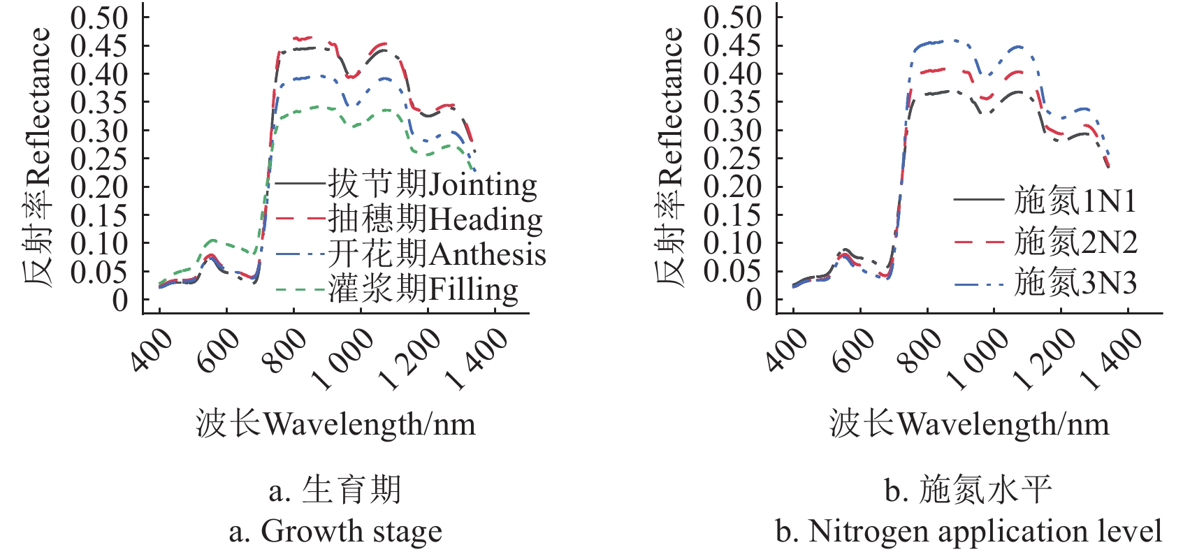
2500 nm。冠层光谱测量时间在当天10:00~14:00之间并选在无风无云的晴朗天气开展。测量时光谱仪垂直于冬小麦冠层上方约1 m处,每个田块选取3个采样点,每个采样点进行3次重复测量,以平均值作为田块冠层光谱。每次冠层光谱测量前进行标准白板校正,测量光谱为冠层光谱反射率。对原始光谱反射率采用Savitzky-Golay方法进行滤波处理降低噪声干扰。考虑到光谱反射率对SPAD值的敏感性波段,本研究中使用的光谱范围为400~1340 nm。图1中展示了不同生育期和施氮水平条件下的所用6个冬小麦品种的平均冠层光谱反射率。![]() 图 1 冬小麦在各生育期和施氮条件下的平均光谱反射率Figure 1. Mean spectral reflectance of winter wheat during each growth stage and under nitrogen application level
图 1 冬小麦在各生育期和施氮条件下的平均光谱反射率Figure 1. Mean spectral reflectance of winter wheat during each growth stage and under nitrogen application level1.4 植被指数
该研究中选取25个常用的叶绿素含量敏感高光谱植被指数,包括两波段比值型、归一化型、三波段型和植被指数组合型等多种类型植被指数。其计算式如表2所示。
表 2 高光谱植被指数Table 2. Hyperspectral vegetation indices植被指数
Vegetation indices参考文献
ReferencesPRI = (r550−r531)/(r550−r531)(r550−r531)(r550−r531) [20] SRPI = r450/r680 [21] CARI = [(r700−r670) - 0.2(r700−r550)] [22] SIPI = (r800−r450)/(r800−r450)(r800−r680)(r800−r680) [23] OSAVI = [(1 + 0.16)(r800−r670)]/[(1 + 0.16)*(r800−r670)](r800 + r670 + 0.16)(r800 + r670 + 0.16) [24] mTVI(red - edge) = 60(r800−r550) - 100(r720−r550) [25] PSSRα = r800/r800r680r680 [26] MCARI = [(r700−r670) - 0.2(r700−r550)](r700/r700r670r670) [27] MCARI/MCARIOSAVIOSAVI = [(r700−r670) - 0.2(r700−r550)](r700/r700r670r670)[(1 + 0.16)(r800−r670)]/[(1 + 0.16)*(r800−r670)](r800 + r670 + 0.16)(r800 + r670 + 0.16) [27] HDVI = (r827−r668)/(r827−r668)(r827 + r668)(r827 + r668) [28] TCARI = 3[(r700−r670) - 0.2(r700−r550)(r700/r700r670r670)] [29] TCARI/TCARIOSAVIOSAVI = 3[(r700−r670) - 0.2(r700−r550)(r700/r700r670r670)][(1 + 0.16)(r800−r670)]/[(1 + 0.16)*(r800−r670)](r800 + r670 + 0.16)(r800 + r670 + 0.16) [29] MTCI = (r754−r709)/(r754−r709)(r709−r680)(r709−r680) [30] CI740 = (r780/r780r740r740) - 1 [31] CI705 = (r780/r780r705r705) - 1 [31] TCARI/TCARIOSAVIOSAVI[705,750] = 3[(r750−r705) - 0.2(r750−r550)(r750/r750r705r705)](r750−r705)/(r750−r705)(r750 + r705 + 0.16)(r750 + r705 + 0.16) [32] Green NDVI = (r780−r560)/(r780−r560)(r780 + r560)(r780 + r560) [33] Green chlorophyll index = (r780/r780r560r560) - 1 [31] Red edge NDVI705 = (r780−r705)/(r780−r705)(r780 + r705)(r780 + r705) [33] Red edge NDVI740 = (r780−r740)/(r780−r740)(r780 + r740)(r780 + r740) [33] Double difference index(DD) = (r750−r720)−(r700−r670) [34] Modified normalized difference(mND705) = (r750−r705)/(r750−r705)(r750 + r705 - 2*r450)(r750 + r705 - 2r450) [35] Triangular vgetation index(TVI) = 60(r800−r560) - 100(r680−r560) [25] Modified simple ratio(mSR705) = (r750−r450)/(r750−r450)(r750 + r450)(r750 + r450) [35] Normalized difference vegetation index(NDVI) = (r800−r680)/(r800−r680)(r800 + r680)(r800 + r680) [36] 注:r为波段,下标为波长。 Note: The r indicates the band and the subscript is the wavelength. 1.5 光谱分辨率重采样
依据现有光学遥感平台所搭载的光学传感器,包括地基光谱仪(1 nm),无人机、航空和卫星所搭载的高光谱(5~10 nm)、多光谱传感器(15~50 nm) 常用的光谱尺度。本研究中,以原始1 nm光谱反射率为基础,采用高斯分布光谱响应函数模拟了5、10、25 和50 nm光谱分辨率的反射率,其计算式如下:
ρj=λe(j)∫λs(j)ρ(λ)Sj(λ)dλ/λe(j)∫λs(j)ρ(λ)Sj(λ)dλλe(j)∫λs(j)Sj(λ)dλλe(j)∫λs(j)Sj(λ)dλ (1) 其中ρj为重采样后的第j波段的冠层反射率,ρ(λ)为原始的光谱数据,λ为波长(nm),λs(j)和λe(j)为波段j的起始波长和终止波长(nm),Sj(λ)为用于波段j重采样的光谱响应函数,dλ为积分步长。高斯光谱响应函数计算式如下:
Sj(λ)=exp{−(λ−cjFWHMk2√ln2)2} (2) 式中cj为波段j的中心波长(nm),FWHMk(full width half maximum)为模拟的光谱尺度。
1.6 机器学习算法
本研究中采用随机森林回归(random forest regression, RFR)、支持向量回归(support vector regression, SVR)和偏最小二乘回归(partial least squares regression, PLSR)3种机器学习算法构建叶片SPAD估算模型。以叶片SPAD值为因变量,以不同光谱尺度的植被指数为自变量,在每种光谱尺度下,分别以与SPAD决定系数最佳的5、10、15和20个植被指数以及全部植被指数作为模型输入,通过优化输入特征构建最佳估算模型。采用留一法交叉验证评估模型精度,并利用网格搜索法优化超参数。
1.6.1 随机森林回归
随机森林回归是由Breiman在2001年提出的一种集成学习算法[37]。对随机森林算法中的两个超参数进行优化,包括森林中树的数量(ntree)和每个节点上随机子集中的特征数量(mtry)[38]。本研究中参数ntree的取值范围为20~2 000,参数mtry的取值范围为1~20。
1.6.2 支持向量回归
支持向量机是一种基于核函数的模型,用于多维空间中的分类、回归和函数逼近[39]。本研究中采用径向基核函数,同时对核参数(gamma)和惩罚系数(C)进行优化,超参数gamma的变化范围为0.001~1,C的变化范围为5~
5000 。1.6.3 偏最小二乘回归
偏最小二乘回归融合了多元线性回归分析、典型相关分析和主成分分析的优势。当样本量较小,且变量之间存在多元相关性时,PLSR方法比传统的回归模型更具优势。PLSR技术将识别出几个线性独立的新变量来替代以前的自变量,使自变量之间的多样性最大化,并缓解过拟合问题,它可以处理多维和共线的数据集[40]。本研究对主成分个数n_components进行优化,参数范围为2~20。
1.7 精度评价与敏感性分析
采用决定系数(R2)和均方根误差(RMSE)进行精度评价。R2值可以表征变量间的拟合程度,该值在0~1之间变化,数值越大表示拟合效果越好。RMSE可以衡量实测值和估计值之间的差异,该值越小表示实测值和估计值越接近。单波段反射率和植被指数对SPAD的敏感性通过光谱尺度敏感性变异系数(Var)衡量,该值越大表示波段反射率或植被指数对SPAD的敏感性受到光谱尺度的影响越大,其计算式如下,其中Rmax和 R_{\min }^2 分别为波段反射率或植被指数在不同光谱尺度下对SPAD的决定系数的最大值和最小值。
{\text{Var}} = \frac{{R_{\max }^2 - R_{\min }^2}}{{R_{\max }^2}} (3) 2. 结果与分析
2.1 不同光谱尺度单波段光谱反射率对SPAD敏感性
图2和表3中展示了构建25个植被指数所用的12个主要单波段反射率在5种光谱尺度下对SPAD的敏感性,包括蓝光波段反射率(中心波长450 nm),绿光波段反射率(中心波长530 和550 nm),红光波段反射率(中心波长680 nm),红边波段反射率(中心波长700~750 nm)和近红外波段反射率(中心波长780、800 和 830 nm)。在全生育期中,红光波段反射率对SPAD的敏感性最大,在5种光谱尺度下决定系数R2在0.411~0.579。红边波段730 nm反射率对SPAD的敏感性最低,R2在0.040~0.062。红边波段710 nm反射率的光谱尺度敏感性变异系数最大,Var为1.000。在4个单一生育期中,红光波段反射率的敏感性最高,单一生育期中敏感性最佳的光谱尺度对应的R2在0.242~0.700。在灌浆期敏感性最高,最佳光谱尺度为1 nm,抽穗期敏感性最低,对应的光谱尺度为25 nm。红边波段730 nm反射率的敏感性最低,单一生育期中敏感性最佳光谱尺度对应的R2在0.021~0.162之间。在3种施氮水平条件下,红光波段反射率的敏感性最高,不同施氮水平条件下的敏感性最佳光谱尺度对应的R2在0.493~0.600,在N1条件下的敏感性最高,而在N3条件下最低,对应的最佳光谱尺度为1 ~10 nm。红边波段730 nm反射率的敏感性最低,最佳光谱尺度(50 nm)对应的R2在0.028~0.077。
![]() 图 2 单波段光谱反射率与SPAD值在5种不同光谱尺度下的决定系数Figure 2. Determination coefficients between individual band reflectance and SPAD value at five spectral scales表 3 单波段光谱反射率与植被指数在不同生育期和施氮水平条件的敏感性变异系数Table 3. Coefficient of sensitivity variation for single band spectral reflectance and vegetation indices at different growth stage and nitrogen application level
图 2 单波段光谱反射率与SPAD值在5种不同光谱尺度下的决定系数Figure 2. Determination coefficients between individual band reflectance and SPAD value at five spectral scales表 3 单波段光谱反射率与植被指数在不同生育期和施氮水平条件的敏感性变异系数Table 3. Coefficient of sensitivity variation for single band spectral reflectance and vegetation indices at different growth stage and nitrogen application level中心波段/植被指数
Central wavelength/
Vegetation index全生育期
ALL施氮1
N1施氮2
N2施氮3
N3拔节期
Jointing抽穗期
Heading开花期
Anthesis灌浆期
Filling450 nm 0.114 0.121 0.134 0.076 0.133 0.466 0.087 0.187 530 nm 0.522 0.550 0.537 0.629 0.364 1.000 0.441 0.732 550 nm 0.654 0.683 0.663 0.761 0.561 1.000 0.507 0.813 680 nm 0.497 0.507 0.544 0.567 0.656 0.952 0.313 0.676 700 nm 0.964 0.959 0.943 0.983 0.992 0.981 0.969 0.941 710 nm 1.000 1.000 0.997 1.000 1.000 1.000 1.000 0.997 730 nm 0.583 0.279 0.554 0.602 0.990 0.389 0.954 0.199 740 nm 0.389 0.429 0.549 0.388 0.153 0.019 0.084 0.564 750 nm 0.398 0.378 0.510 0.420 0.487 0.111 0.371 0.543 780 nm 0.089 0.079 0.108 0.104 0.193 0.037 0.127 0.150 800 nm 0.012 0.017 0.012 0.012 0.044 0.005 0.021 0.028 830 nm 0.001 0.011 0.005 0.009 0.015 0.005 0.001 0.017 mND705 0.014 0.043 0.015 0.027 0.021 0.102 0.071 0.029 NDVI 0.087 0.052 0.041 0.062 0.093 0.070 0.163 0.062 HNDVI 0.007 0.030 0.014 0.029 0.063 0.068 0.119 0.048 Red edge NDVI705 0.056 0.075 0.043 0.032 0.007 0.073 0.039 0.005 SIPI 0.107 0.175 0.218 0.047 0.182 0.092 0.320 0.233 Green NDVI 0.072 0.067 0.070 0.057 0.027 0.047 0.017 0.047 OSAVI 0.104 0.019 0.038 0.030 0.126 0.063 0.128 0.084 MTCI 0.302 0.358 0.390 0.342 0.118 0.142 0.053 0.195 Red edge NDVI740 0.400 0.519 0.594 0.580 0.097 0.293 0.155 0.352 CI740 0.455 0.515 0.594 0.575 0.122 0.292 0.176 0.365 mSR705 0.496 0.534 0.613 0.634 0.197 0.155 0.119 0.218 CI705 0.385 0.407 0.491 0.512 0.137 0.098 0.089 0.203 Green chlorophyll index 0.076 0.002 0.041 0.100 0.030 0.029 0.015 0.039 DD 0.071 0.072 0.183 0.153 0.074 0.055 0.061 0.058 mTVI 0.027 0.149 0.125 0.071 0.218 0.023 0.105 0.055 SRPI 0.154 0.807 0.418 0.374 0.967 0.406 0.662 0.505 TVI 0.264 0.085 0.218 0.203 0.378 0.109 0.253 0.286 TCARI/OSAVI 0.266 0.990 1.000 1.000 0.250 0.972 0.724 0.979 PSSRα 0.648 0.365 0.591 0.699 0.259 0.212 0.282 0.143 TCARI/OSAVI[705,750] 0.814 0.714 0.971 1.000 0.894 1.000 0.846 0.862 MCARI/OSAVI 0.927 1.000 0.998 0.999 0.992 0.996 1.000 0.999 MCARI 0.974 0.760 0.993 0.980 0.996 0.766 0.999 0.987 TCARI 0.995 0.963 1.000 0.998 0.996 0.688 1.000 0.986 PRI 1.000 0.979 1.000 1.000 1.000 0.999 0.977 1.000 CARI 1.000 0.992 1.000 1.000 1.000 0.955 0.998 0.997 注:敏感性变异系数指在不同光谱尺度下中心波段或植被指数对SPAD的敏感性受到的影响。 Note: The coefficient of variation of sensitivity refers to the influence of the sensitivity of the central band or the vegetation index to SPAD at different spectral scales. 2.2 不同光谱尺度植被指数对SPAD敏感性
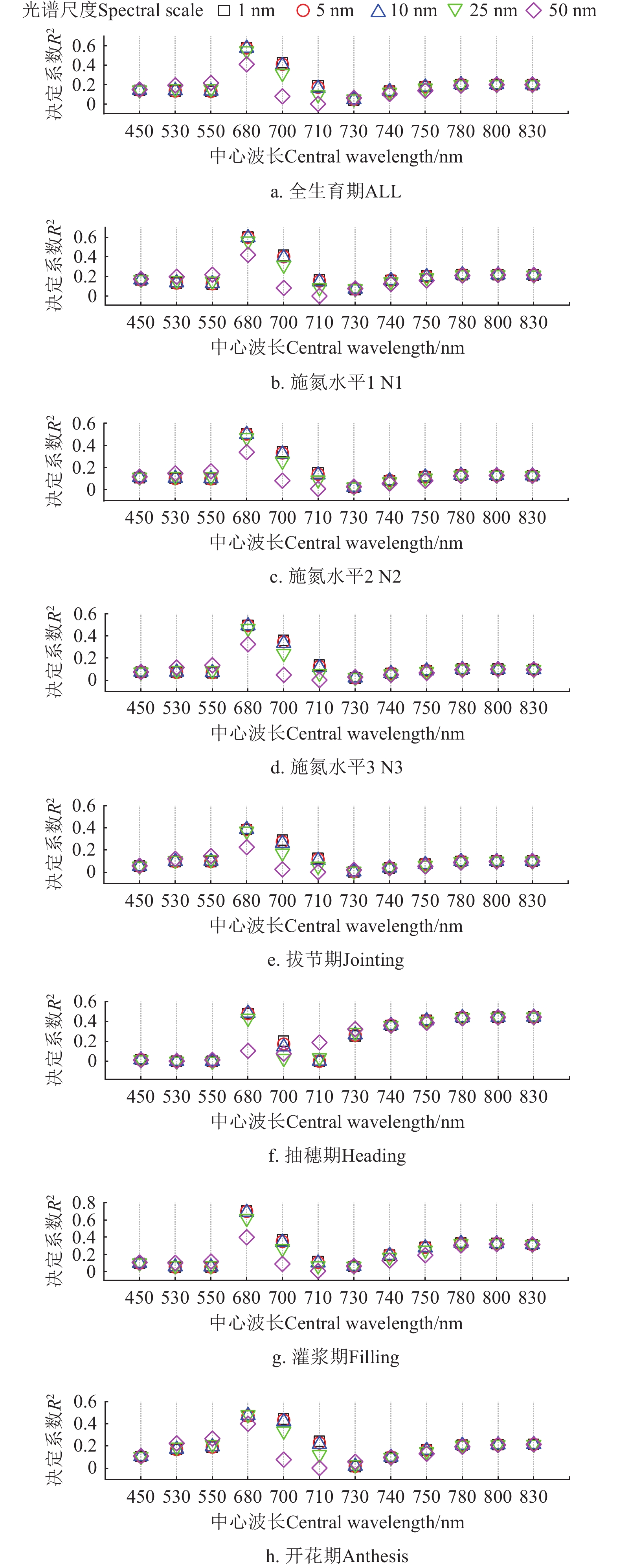
在4个关键生育期和3种施氮水平条件下,不同光谱尺度植被指数与SPAD的决定系数和光谱尺度敏感性变异系数如图3和表3所示。
![]() 图 3 植被指数与SPAD值在5种不同光谱尺度下的决定系数Figure 3. Determination coefficients between vegetation indices and SPAD value at five spectral scale
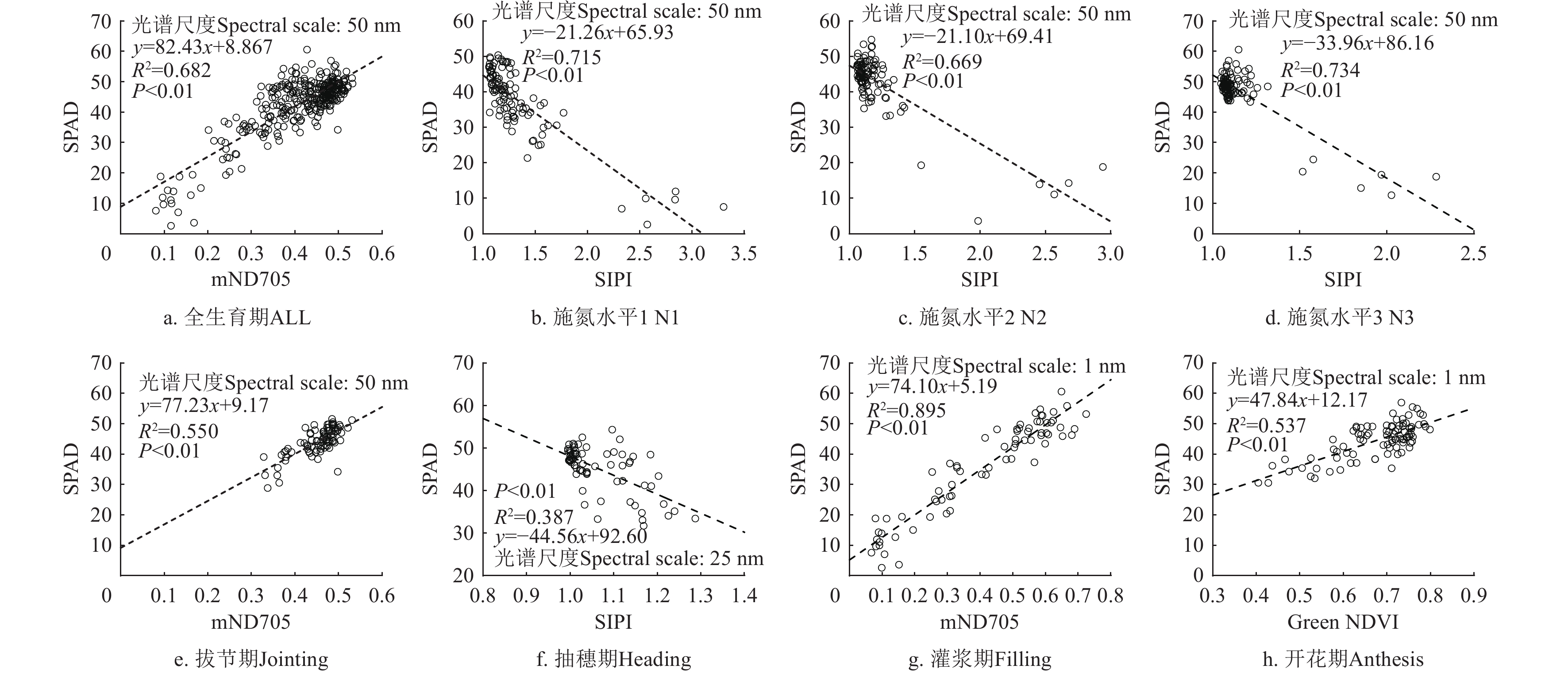
图 3 植被指数与SPAD值在5种不同光谱尺度下的决定系数Figure 3. Determination coefficients between vegetation indices and SPAD value at five spectral scale全生育期中SPAD敏感性最佳植被指数为mND705和SIPI,对应的光谱尺度为50 nm,决定系数R2分别为0.685和0.684,光谱尺度敏感性变异系数Var分别0.014和0.055。在4个单一生育期中,拔节期敏感性最佳植被指数为mND705,对应的光谱尺度为50 nm,决定系数R2为0.550,光谱尺度敏感性变异系数Var为0.011。在抽穗期,敏感性最佳植被指数为SIPI,对应的光谱尺度为25 nm,决定系数R2为0.387,光谱尺度敏感性变异系数Var为0.047。开花期中敏感性最佳植被指数为Green NDVI,对应的光谱尺度为1 nm,决定系数R2为0.537,Var为0.009。在灌浆期,敏感性最佳植被指数为mND705,对应的光谱尺度为1 nm,决定系数为0.895,光谱尺度敏感性变异系数Var为0.014。在3种施氮水平条件下,SIPI对SPAD的敏感性最佳,对应的光谱尺度为50 nm,决定系数R2在0.669~0.734,Var在0.024~0.116之间。图4中展示了单一生育期和不同施氮水平条件下敏感性最佳光谱尺度及植被指数与SPAD的相关关系。其中在全生育期,拔节期,开花期和灌浆期二者成正相关关系,在抽穗期和其他3个单一施氮水平中都成负相关关系。
![]() 图 4 不同生育期和施氮水平条件下敏感性最佳植被指数及光谱尺度与冬小麦SPAD相关关系Figure 4. Relationship between optimal spectral indices at the corresponding spectral scale and SPAD value under different growth stage and nitrogen application level
图 4 不同生育期和施氮水平条件下敏感性最佳植被指数及光谱尺度与冬小麦SPAD相关关系Figure 4. Relationship between optimal spectral indices at the corresponding spectral scale and SPAD value under different growth stage and nitrogen application level2.3 光谱尺度对机器学习模型估算SPAD的影响
表4中展示了5种光谱尺度植被指数结合机器学习估算SPAD的精度。在全生育期中,PLSR模型在25 nm光谱尺度估算精度最佳,决定系数R2为0.816和RMSE为4.04。在4个单一生育期中,最佳光谱尺度在1和50 nm,模型精度R2=0.531~0.916和RMSE=2.76~4.47。拔节期中1 nm光谱尺度的SVR模型估算精度最佳,决定系数R2为0.618和RMSE为2.86。在抽穗期,在50 nm光谱尺度的PLSR模型估算精度最佳,决定系数R2为0.733和RMSE为2.76。开花期中50 nm光谱尺度的估算精度最佳,决定系数R2为0.531和RMSE为3.99。在灌浆期,在1 nm光谱尺度的估算精度最佳,决定系数R2为0.916和RMSE为4.47。在3种施氮水平条件下,最佳光谱尺度均为50 nm,模型精度R2在0.780~0.884,RMSE在2.67~4.55之间。
表 4 各生育期及3种施氮条件下基于机器学习的冬小麦SPAD值估算精度Table 4. SPAD estimation at each growth stage and three nitrogen application level with machine learning光谱尺度
Spectral
scale/nm模型
Model全生育期
ALL拔节期
Jointing抽穗期
Heading开花期
Anthesis灌浆期
Filling施氮1
N1施氮2
N2施氮3
N3R2 RMSE R2 RMSE R2 RMSE R2 RMSE R2 RMSE R2 RMSE R2 RMSE R2 RMSE 1 RFR 0.800 4.20 0.563 3.05 0.544 3.57 0.454 4.33 0.895 4.99 0.770 4.66 0.785 3.88 0.868 2.79 SVR 0.806 4.14 0.618 2.86 0.616 3.29 0.515 4.06 0.908 4.68 0.706 5.26 0.820 3.54 0.844 3.13 PLSR 0.813 4.10 0.569 3.05 0.679 3.05 0.520 4.03 0.916 4.47 0.755 4.80 0.791 3.82 0.859 2.87 5 RFR 0.803 4.17 0.573 3.02 0.536 3.62 0.464 4.28 0.887 5.19 0.766 4.70 0.781 3.91 0.863 2.82 SVR 0.804 4.16 0.615 2.88 0.619 3.29 0.521 4.04 0.908 4.66 0.763 4.72 0.819 3.56 0.842 3.16 PLSR 0.813 4.11 0.572 3.03 0.673 3.08 0.517 4.05 0.914 4.52 0.755 4.80 0.790 3.84 0.857 2.88 10 RFR 0.801 4.20 0.563 3.05 0.515 3.70 0.465 4.29 0.882 5.29 0.764 4.71 0.785 3.88 0.871 2.76 SVR 0.791 4.30 0.490 3.31 0.643 3.18 0.524 4.02 0.909 4.64 0.726 5.08 0.813 3.62 0.876 2.70 PLSR 0.813 4.09 0.560 3.08 0.677 3.05 0.513 4.07 0.914 4.51 0.764 4.77 0.790 3.83 0.856 2.89 25 RFR 0.793 4.28 0.581 2.99 0.521 3.66 0.463 4.29 0.890 5.11 0.746 4.90 0.777 3.95 0.874 2.72 SVR 0.802 4.18 0.539 3.25 0.621 3.28 0.522 4.03 0.900 4.88 0.711 5.26 0.817 3.66 0.872 2.74 PLSR 0.816 4.04 0.558 3.09 0.709 2.88 0.506 4.10 0.915 4.48 0.774 4.65 0.799 3.75 0.858 2.88 50 RFR 0.787 4.34 0.587 2.97 0.527 3.65 0.444 4.38 0.879 5.36 0.754 4.82 0.791 3.86 0.884 2.67 SVR 0.800 4.21 0.503 3.26 0.589 3.39 0.493 4.16 0.903 4.81 0.780 4.55 0.827 3.51 0.807 3.37 PLSR 0.807 4.13 0.560 3.07 0.733 2.76 0.531 3.99 0.913 4.56 0.770 4.66 0.808 3.67 0.851 2.95 在N1施氮水平条件下,SVR算法所构建的估算精度最佳,决定系数R2为0.780和RMSE为4.55。N2施氮条件下SVR算法的估算精度最佳,决定系数R2为0.827和RMSE为3.51。在N3施氮条件下,RF算法的估算精度最佳,决定系数R2为0.884和RMSE为2.67。图5中展示了不同生育期和施氮水平条件下最佳估算模型实测与预测SPAD相关关系。
![]() 图 5 不同生育期和施氮水平条件下最佳光谱尺度与机器学习算法估算SPAD值与实测值相关关系Figure 5. SPAD estimation based on optimal spectral scale and machine learning algorithms at different growth stage and nitrogen application level
图 5 不同生育期和施氮水平条件下最佳光谱尺度与机器学习算法估算SPAD值与实测值相关关系Figure 5. SPAD estimation based on optimal spectral scale and machine learning algorithms at different growth stage and nitrogen application level3. 讨 论
冬小麦叶片SPAD值反映了叶片叶绿素相对含量,是监测冬小麦长势和营养状况的重要指标。光学遥感是快速、无损探测叶片SPAD值的重要手段。不同类型的光学遥感传感器不仅在获取光学信号通道位置上存在差异,所获取光信号的光谱尺度也不一致,增加了光学遥感探测叶片SPAD的不确定性。准确评估光谱尺度对叶片SPAD值遥感探测的影响,是进一步优化传感器设计,提升叶片SPAD光学探测精度的基础。
单一波段反射率对SPAD的敏感性受到光谱尺度、生育期和施氮水平的影响。在全生育期中,红光波段反射率对SPAD的敏感性最大,在5种光谱尺度下决定系数R2在0.411~0.579,与前人报道的无人机获取的红光波段反射率对SPAD的敏感性一致(R2=0.460)[41],但高于Sentinel-2卫星红光波段反射率的敏感性(R2=0.255)[42]。这主要是由于叶绿素对红光波段的强吸收作用。在不同生育期中的敏感性最佳光谱尺度下,R2在0.242~0.700,这与牛庆林等[41]采用无人机RGB多光谱影像获取的结果一致,Var在0.313~0.952。 在710 nm处的红边波段反射率的光谱尺度敏感性变异系数最大,在全生育期中Var=1.000,主要原因是健康植被在红边波段反射率急剧变化,不同光谱尺度的反射率存在明显差异。
如图1所示,施氮水平的增加在不同程度上降低了400~700 nm波段的反射率而增加了近红外波段的反射率。主要原因是随着施氮水平的提升叶片叶绿素含量(SPAD值)随之增加,进而增加了对可见光波段反射率(特别是蓝光和红光波段)的吸收。同时是施氮水平的提升促进了植株的生长,叶面积指数随之增大进而增强了近红外波段的反射率。JACQUEMOUD等[43]通过冠层辐射传输模型PROSAIL模拟了全波段光谱反射率对冠层生理生化参数的响应,在400 ~ 700 nm波段范围内反射率主要(50%以上)由叶绿素含量决定,其次为冠层平均叶倾角和叶片结构参数。而在700 ~ 730 nm波段范围内,叶绿素含量对反射率的贡献由大约65%快速下降到约30%,而冠层平均叶倾角和叶面积指数对反射率的贡献分别由5%以下上升到25%以上。而在730 ~ 750 nm范围内,叶绿素含量对反射率的影响由30%左右急剧下降,在波长大于750 nm范围内的波段反射率不受叶绿素含量影响。通过辐射传输模拟进一步解释了SPAD对红边波段反射率敏感性受到光谱尺度影响较大,而对近红外波段反射率敏感性几乎不受光谱尺度影响。
在不同生育期和施氮水平条件下光谱尺度影响了植被指数对SPAD的敏感性。除灌浆期和开花期外,敏感性最佳植被指数的光谱尺度范围在25~50 nm,可能的原因是对于敏感性最佳植被指数,光谱尺度范围的增大使植被指数包含了更多的光谱信息并降低了噪声的影响,但与单波段反射率对SPAD的敏感性受到光谱尺度的影响相比,敏感性最佳植被指数对SPAD的敏感性受到光谱尺度的影响有限。在全生育期中,敏感性最佳植被指数mND705在50 nm对SPAD的敏感性最高,R2为0.685 且光谱尺度敏感性变异系数低Var=0.014,高于高分一号卫星数据构建的最佳植被指数对SPAD的敏感性(R2=0.230)[44]。在4个单一生育期中,受到不同生育期的影响,敏感性最佳植被指数的敏感性R2在0.387~0.895之间,但受到光谱尺度的影响较小,敏感性变异系数Var在0.01~0.05,这与高分一号卫星数据[44]和模拟的RapidEye[45]卫星宽波段植被指数的结果较为一致(R2范围分别在0.550 ~ 0.620和0.450 ~ 0.690),但高于无人机高植被指数在不同生育期的敏感性(R2=0.291~0.555)[46]。在3种施氮水平条件下,与SPAD敏感性最佳植被指数均为3波段植被指数SIPI,该植被指数同时利用了与SPAD敏感的蓝光波段(450 nm)和红光波段(680 nm)以及与冠层结构参数敏感的近红外波段(800 nm)反射率,通过3个波段的组合突出了对SPAD的敏感性并降低了冠层结构的影响。
优化光谱尺度作为机器学习模型输入特征提升了SPAD的估算精度。在全生育期中,以25 nm光谱尺度植被指数所构建PLSR模型对SPAD的估算精度最佳,实测与预测值的决定系数R2为0.816,高于高分一号卫星多光谱数据[44]和无人机高光谱数据[47]结合机器学习估算SPAD的决定系数(R2分别为0.660和0.734)。在50 nm光谱尺度下,PLSR模型对SPAD估算的实测与预测值的决定系数R2为0.807,与相似光谱尺度下无人机估算SPAD的决定系数一致(R2=0.807)[10]。WANG等 [13]采用光谱尺度在16 ~ 26 nm无人机多光谱数据结合支持向量回归估算不同水分胁迫条件下冬小麦叶片SPAD值,在不同生育期决定系数R2在0.350~0.660之间,低于本研究中相似光谱尺度(10 ~ 25 nm )在不同生育期的决定系数(R2在0.520~0.920之间)。不同生育期SPAD最佳估算模型所用光谱尺度存在明显差异,在拔节期和灌浆期为1 nm而在抽穗期和开花期为 50 nm。总体上,在单一生育期内,随着光谱尺度的增加对SPAD的估算精度呈现出先降低而后增加的趋势。在拔节期内,1 nm 光谱尺度估算精度最佳,5 nm光谱尺度降低了估算精度,而在 10 nm光谱尺度估算精度最低,而25 和50 nm光谱尺度估算精度逐步提升。在抽穗期和开花期,5 nm 光谱尺度下估算精度最低,且随着光谱尺度的增加估算精度逐步提升,在50 nm光谱尺度估算精度最佳。在灌浆期内,1 nm 光谱尺度估算精度最佳而5 nm光谱尺度估算精度最低,而随着光谱尺度增加估算精度逐步提升。因而,全生育期中最佳光谱尺度为单一生育期中最佳光谱尺度的均值(25 nm),这与通过辐射传输模型模拟叶绿素含量估算最佳光谱尺度在10 ~ 30 nm较为一致[48]。在3种施氮水平条件下,以最佳光谱尺度所构建模型对SPAD的估算精度R2在0.780~0.884之间,RMSE在2.67~4.55。施氮水平的提升提高了叶片叶绿素含量,进而增强了基于光谱特征的机器学习模型对SPAD的探测能力。总体上,在单一施氮水平中,与在单一生育期内较为相似,随着光谱尺度的增加对SPAD的估算精度同样呈现出先降低而后增加的趋势,并且在 50 nm光谱尺度估算精度最佳。
在4个单一生育期中,如图5所示,灌浆期的决定系数(R2=0.916)要高于其他3个生育期(R2=0.531 ~ 0.733),主要原因是灌浆期SPAD值变化范围要明显大于其他3个生育期,使实测SPAD值与其均值之间的差的平方和明显大于其他3个生育期,根据决定系数的计算式,计算出的决定系数要大于其他3个生育期。灌浆期SPAD变化范围较大的潜在原因是冬小麦不同品种在关键生育期长势存在差异,特别是在灌浆中后期不同品种叶绿素含量、净光合速率和黄化速率会出现明显差异[49]。在实际农业生产中,冬小麦品种多样且种植范围灵活,品种的差异性增加了对一些关键生育期SPAD遥感估算的不确定性。
该研究的局限性在于采用近地光谱测量获取冬小麦冠层光谱反射率,通过对原始1 nm光谱反射率重采样分析SPAD遥感的光谱尺度效应。对于航空或航天遥感观测平台获取的光谱数据会受到大气和地表混合像元等因素的影响,这些因素对SPAD的光谱尺度效应的影响在未来的研究中需要进一步评估。此外,该研究所获取数据年份为2011—2014年,在未来的研究中需要获取新的数据进一步评估和验证算法精度。
4. 结 论
本研究通过4年田间试验,评估了冬小麦在4个关键生育期和3种施氮水平条件下光谱尺度对单波段反射率、植被指数对叶片SPAD(soil and plant analyzer development)的敏感性及对机器学习模型估算SPAD的影响。本研究主要有以下结论:
1)对单波段光谱反射率,红光波段对SPAD的敏感性最大,而红边波段730 nm对SPAD的敏感性最低。在全生育期植被指数mND705对SPAD敏感性最佳(R2 = 0.685)且受到光谱尺度的影响小(Var=0.014)。在4个单一生育期中,mND705在灌浆期对SPAD的敏感性最佳(R2=0.895)且受到光谱尺度的影响小(Var=0.01)。在 3种施氮水平条件下,植被指数SIPI与SPAD的敏感性最佳(R2=0.669~0.734)且光谱敏感性变异系数Var=0.024~0.116。
2)光谱尺度影响了机器学习估算SPAD的精度。在全生育期中,以25 nm光谱尺度构建的PLSR估算模型精度最佳,决定系数R2为0.816和RMSE为4.04,优化光谱尺度提升了模型估算精度。在未来的研究中需要进一步评估光谱尺度对不同作物类型、不同生长环境条件下叶绿素含量及其他养分含量探测的影响。
-
![]()
图 1 冬小麦在各生育期和施氮条件下的平均光谱反射率
Figure 1. Mean spectral reflectance of winter wheat during each growth stage and under nitrogen application level
![]()
图 2 单波段光谱反射率与SPAD值在5种不同光谱尺度下的决定系数
Figure 2. Determination coefficients between individual band reflectance and SPAD value at five spectral scales
![]()
图 3 植被指数与SPAD值在5种不同光谱尺度下的决定系数
Figure 3. Determination coefficients between vegetation indices and SPAD value at five spectral scale
![]()
图 4 不同生育期和施氮水平条件下敏感性最佳植被指数及光谱尺度与冬小麦SPAD相关关系
Figure 4. Relationship between optimal spectral indices at the corresponding spectral scale and SPAD value under different growth stage and nitrogen application level
![]()
图 5 不同生育期和施氮水平条件下最佳光谱尺度与机器学习算法估算SPAD值与实测值相关关系
Figure 5. SPAD estimation based on optimal spectral scale and machine learning algorithms at different growth stage and nitrogen application level
表 1 试验基本信息
Table 1 Basic information of the test
年份
Year品种
Variety施氮水平
Nitrogen application level样本数量
Number of samples2011 徐麦31 和宁麦12 N1、N2、N3 72 2012 扬麦13 和镇麦168 90 2013 扬麦13和扬麦16 72 2014 扬麦13 和宁麦13 88  下载: 导出CSV
表 2 高光谱植被指数
Table 2 Hyperspectral vegetation indices
植被指数
Vegetation indices参考文献
References{\text{PRI = }}{{\left( {{r_{{\text{550}}}} - {r_{{\text{531}}}}} \right)} \mathord{\left/ {\vphantom {{\left( {{r_{{\text{550}}}} - {r_{{\text{531}}}}} \right)} {\left( {{r_{{\text{550}}}} - {r_{{\text{531}}}}} \right)}}} \right. } {\left( {{r_{{\text{550}}}} - {r_{{\text{531}}}}} \right)}} [20] {\text{SRPI = }}{r_{{\text{450}}}}{\text{/}}{r_{{\text{680}}}} [21] \text{CARI = }\left[\left(r_{\text{700}}-r_{\text{670}}\right)\text{ - 0}\text{.2}\left(r_{\text{700}}-r_{\text{550}}\right)\right] [22] {\text{SIPI = }}{{\left( {{r_{{\text{800}}}} - {r_{{\text{450}}}}} \right)} \mathord{\left/ {\vphantom {{\left( {{r_{{\text{800}}}} - {r_{{\text{450}}}}} \right)} {\left( {{r_{{\text{800}}}} - {r_{{\text{680}}}}} \right)}}} \right. } {\left( {{r_{{\text{800}}}} - {r_{{\text{680}}}}} \right)}} [23] \text{OSAVI = }\left[\left(\text{1 + 0}\text{.16}\right)\left(r_{\text{800}}-r_{\text{670}}\right)\right]\mathord{\left/\vphantom{\left[\left(\text{1 + 0}\text{.16}\right)\text{*}\left(r_{\text{800}}-r_{\text{670}}\right)\right]\left(r_{\text{800}}\text{ + }r_{\text{670}}\text{ + 0}\text{.16}\right)}\right.}\left(r_{\text{800}}\text{ + }r_{\text{670}}\text{ + 0}\text{.16}\right) [24] \text{mTVI}\left(\text{red - edge}\right)\text{ = 60}\left(r_{\text{800}}-r_{\text{550}}\right)\text{ - 100}\left(r_{\text{720}}-r_{\text{550}}\right) [25] {\text{PSS}}{{\text{R}}_{\text{α }}}{\text{ = }}{{{r_{{\text{800}}}}} \mathord{\left/ {\vphantom {{{r_{{\text{800}}}}} {{r_{{\text{680}}}}}}} \right. } {{r_{{\text{680}}}}}} [26] \text{MCARI = }\left[\left(r_{\text{700}}-r_{\text{670}}\right)\text{ - 0}\text{.2}\left(r_{\text{700}}-r_{\text{550}}\right)\right]\left(r_{\text{700}}\mathord{\left/\vphantom{r_{\text{700}}r_{\text{670}}}\right.}r_{\text{670}}\right) [27] \text{MCARI}\mathord{\left/\vphantom{\text{MCARI}\text{OSAVI}}\right.}\text{OSAVI}\text{ = }\dfrac{\left[\left(r_{\text{700}}-r_{\text{670}}\right)\text{ - 0}\text{.2}\left(r_{\text{700}}-r_{\text{550}}\right)\right]\left(r_{\text{700}}\mathord{\left/\vphantom{r_{\text{700}}r_{\text{670}}}\right.}r_{\text{670}}\right)}{\left[\left(\text{1 + 0}\text{.16}\right)\left(r_{\text{800}}-r_{\text{670}}\right)\right]\mathord{\left/\vphantom{\left[\left(\text{1 + 0}\text{.16}\right)\text{*}\left(r_{\text{800}}-r_{\text{670}}\right)\right]\left(r_{\text{800}}\text{ + }r_{\text{670}}\text{ + 0}\text{.16}\right)}\right.}\left(r_{\text{800}}\text{ + }r_{\text{670}}\text{ + 0}\text{.16}\right)} [27] {\text{HDVI = }}{{\left( {{r_{{\text{827}}}} - {r_{{\text{668}}}}} \right)} \mathord{\left/ {\vphantom {{\left( {{r_{{\text{827}}}} - {r_{{\text{668}}}}} \right)} {\left( {{r_{{\text{827}}}}{\text{ + }}{r_{{\text{668}}}}} \right)}}} \right. } {\left( {{r_{{\text{827}}}}{\text{ + }}{r_{{\text{668}}}}} \right)}} [28] \text{TCARI = 3}\left[\left(r_{\text{700}}-r_{\text{670}}\right)\text{ - 0}\text{.2}\left(r_{\text{700}}-r_{\text{550}}\right)\left(r_{\text{700}}\mathord{\left/\vphantom{r_{\text{700}}r_{\text{670}}}\right.}r_{\text{670}}\right)\right] [29] \text{TCARI}\mathord{\left/\vphantom{\text{TCARI}\text{OSAVI}}\right.}\text{OSAVI}\text{ = }\dfrac{\text{3}\left[\left(r_{\text{700}}-r_{\text{670}}\right)\text{ - 0}\text{.2}\left(r_{\text{700}}-r_{\text{550}}\right)\left(r_{\text{700}}\mathord{\left/\vphantom{r_{\text{700}}r_{\text{670}}}\right.}r_{\text{670}}\right)\right]}{\left[\left(\text{1 + 0}\text{.16}\right)\left(r_{\text{800}}-r_{\text{670}}\right)\right]\mathord{\left/\vphantom{\left[\left(\text{1 + 0}\text{.16}\right)\text{*}\left(r_{\text{800}}-r_{\text{670}}\right)\right]\left(r_{\text{800}}\text{ + }r_{\text{670}}\text{ + 0}\text{.16}\right)}\right.}\left(r_{\text{800}}\text{ + }r_{\text{670}}\text{ + 0}\text{.16}\right)} [29] {\text{MTCI = }}{{\left( {{r_{{\text{754}}}} - {r_{{\text{709}}}}} \right)} \mathord{\left/ {\vphantom {{\left( {{r_{{\text{754}}}} - {r_{{\text{709}}}}} \right)} {\left( {{r_{{\text{709}}}} - {r_{{\text{680}}}}} \right)}}} \right. } {\left( {{r_{{\text{709}}}} - {r_{{\text{680}}}}} \right)}} [30] {\text{C}}{{\text{I}}_{{\text{740}}}}{\text{ = }}\left( {{{{r_{{\text{780}}}}} \mathord{\left/ {\vphantom {{{r_{{\text{780}}}}} {{r_{{\text{740}}}}}}} \right. } {{r_{{\text{740}}}}}}} \right){\text{ - 1}} [31] {\text{C}}{{\text{I}}_{{\text{705}}}}{\text{ = }}\left( {{{{r_{{\text{780}}}}} \mathord{\left/ {\vphantom {{{r_{{\text{780}}}}} {{r_{{\text{705}}}}}}} \right. } {{r_{{\text{705}}}}}}} \right){\text{ - 1}} [31] \text{TCARI}\mathord{\left/\vphantom{\text{TCARI}\text{OSAVI}}\right.}\text{OSAVI}_{\left[\text{705,750}\right]}\text{ = }\dfrac{\text{3}\left[\left(r_{\text{750}}-r_{\text{705}}\right)\text{ - 0}\text{.2}\left(r_{\text{750}}-r_{\text{550}}\right)\left(r_{\text{750}}\mathord{\left/\vphantom{r_{\text{750}}r_{\text{705}}}\right.}r_{\text{705}}\right)\right]}{\left(r_{\text{750}}-r_{\text{705}}\right)\mathord{\left/\vphantom{\left(r_{\text{750}}-r_{\text{705}}\right)\left(r_{\text{750}}\text{ + }r_{\text{705}}\text{ + 0}\text{.16}\right)}\right.}\left(r_{\text{750}}\text{ + }r_{\text{705}}\text{ + 0}\text{.16}\right)} [32] {\text{Green NDVI = }}{{\left( {{r_{{\text{780}}}} - {r_{{\text{560}}}}} \right)} \mathord{\left/ {\vphantom {{\left( {{r_{{\text{780}}}} - {r_{{\text{560}}}}} \right)} {\left( {{r_{{\text{780}}}}{\text{ + }}{r_{{\text{560}}}}} \right)}}} \right. } {\left( {{r_{{\text{780}}}}{\text{ + }}{r_{{\text{560}}}}} \right)}} [33] {\text{Green chlorophyll index = }}\left( {{{{r_{{\text{780}}}}} \mathord{\left/ {\vphantom {{{r_{{\text{780}}}}} {{r_{{\text{560}}}}}}} \right. } {{r_{{\text{560}}}}}}} \right){\text{ - 1}} [31] {\text{Red edge NDV}}{{\text{I}}_{{\text{705}}}}{\text{ = }}{{\left( {{r_{{\text{780}}}} - {r_{{\text{705}}}}} \right)} \mathord{\left/ {\vphantom {{\left( {{r_{{\text{780}}}} - {r_{{\text{705}}}}} \right)} {\left( {{r_{{\text{780}}}}{\text{ + }}{r_{{\text{705}}}}} \right)}}} \right. } {\left( {{r_{{\text{780}}}}{\text{ + }}{r_{{\text{705}}}}} \right)}} [33] {\text{Red edge NDV}}{{\text{I}}_{{\text{740}}}}{\text{ = }}{{\left( {{r_{{\text{780}}}} - {r_{{\text{740}}}}} \right)} \mathord{\left/ {\vphantom {{\left( {{r_{{\text{780}}}} - {r_{{\text{740}}}}} \right)} {\left( {{r_{{\text{780}}}}{\text{ + }}{r_{{\text{740}}}}} \right)}}} \right. } {\left( {{r_{{\text{780}}}}{\text{ + }}{r_{{\text{740}}}}} \right)}} [33] {\text{Double difference index}}\left( {{\text{DD}}} \right){\text{ = }}\left( {{r_{{\text{750}}}} - {r_{{\text{720}}}}} \right) - \left( {{r_{{\text{700}}}} - {r_{{\text{670}}}}} \right) [34] \text{Modified normalized difference}\left(\text{mND705}\right)\text{ = }\left(r_{\text{750}}-r_{\text{705}}\right)\mathord{\left/\vphantom{\left(r_{\text{750}}-r_{\text{705}}\right)\left(r_{\text{750}}\text{ + }r_{\text{705}}\text{ - 2*}r_{\text{450}}\right)}\right.}\left(r_{\text{750}}\text{ + }r_{\text{705}}\text{ - 2}r_{\text{450}}\right) [35] \text{Triangular vgetation index}\left(\text{TVI}\right)\text{ = 60}\left(r_{\text{800}}-r_{\text{560}}\right)\text{ - 100}\left(r_{\text{680}}-r_{\text{560}}\right) [25] {\text{Modified simple ratio}}\left( {{\text{mSR705}}} \right){\text{ = }}{{\left( {{r_{{\text{750}}}} - {r_{{\text{450}}}}} \right)} \mathord{\left/ {\vphantom {{\left( {{r_{{\text{750}}}} - {r_{{\text{450}}}}} \right)} {\left( {{r_{{\text{750}}}}{\text{ + }}{r_{{\text{450}}}}} \right)}}} \right. } {\left( {{r_{{\text{750}}}}{\text{ + }}{r_{{\text{450}}}}} \right)}} [35] {\text{Normalized difference vegetation index}}\left( {{\text{NDVI}}} \right){\text{ = }}{{\left( {{r_{{\text{800}}}} - {r_{{\text{680}}}}} \right)} \mathord{\left/ {\vphantom {{\left( {{r_{{\text{800}}}} - {r_{{\text{680}}}}} \right)} {\left( {{r_{{\text{800}}}}{\text{ + }}{r_{{\text{680}}}}} \right)}}} \right. } {\left( {{r_{{\text{800}}}}{\text{ + }}{r_{{\text{680}}}}} \right)}} [36] 注:r为波段,下标为波长。 Note: The r indicates the band and the subscript is the wavelength.
下载: 导出CSV
表 3 单波段光谱反射率与植被指数在不同生育期和施氮水平条件的敏感性变异系数
Table 3 Coefficient of sensitivity variation for single band spectral reflectance and vegetation indices at different growth stage and nitrogen application level
中心波段/植被指数
Central wavelength/
Vegetation index全生育期
ALL施氮1
N1施氮2
N2施氮3
N3拔节期
Jointing抽穗期
Heading开花期
Anthesis灌浆期
Filling450 nm 0.114 0.121 0.134 0.076 0.133 0.466 0.087 0.187 530 nm 0.522 0.550 0.537 0.629 0.364 1.000 0.441 0.732 550 nm 0.654 0.683 0.663 0.761 0.561 1.000 0.507 0.813 680 nm 0.497 0.507 0.544 0.567 0.656 0.952 0.313 0.676 700 nm 0.964 0.959 0.943 0.983 0.992 0.981 0.969 0.941 710 nm 1.000 1.000 0.997 1.000 1.000 1.000 1.000 0.997 730 nm 0.583 0.279 0.554 0.602 0.990 0.389 0.954 0.199 740 nm 0.389 0.429 0.549 0.388 0.153 0.019 0.084 0.564 750 nm 0.398 0.378 0.510 0.420 0.487 0.111 0.371 0.543 780 nm 0.089 0.079 0.108 0.104 0.193 0.037 0.127 0.150 800 nm 0.012 0.017 0.012 0.012 0.044 0.005 0.021 0.028 830 nm 0.001 0.011 0.005 0.009 0.015 0.005 0.001 0.017 mND705 0.014 0.043 0.015 0.027 0.021 0.102 0.071 0.029 NDVI 0.087 0.052 0.041 0.062 0.093 0.070 0.163 0.062 HNDVI 0.007 0.030 0.014 0.029 0.063 0.068 0.119 0.048 Red edge NDVI705 0.056 0.075 0.043 0.032 0.007 0.073 0.039 0.005 SIPI 0.107 0.175 0.218 0.047 0.182 0.092 0.320 0.233 Green NDVI 0.072 0.067 0.070 0.057 0.027 0.047 0.017 0.047 OSAVI 0.104 0.019 0.038 0.030 0.126 0.063 0.128 0.084 MTCI 0.302 0.358 0.390 0.342 0.118 0.142 0.053 0.195 Red edge NDVI740 0.400 0.519 0.594 0.580 0.097 0.293 0.155 0.352 CI740 0.455 0.515 0.594 0.575 0.122 0.292 0.176 0.365 mSR705 0.496 0.534 0.613 0.634 0.197 0.155 0.119 0.218 CI705 0.385 0.407 0.491 0.512 0.137 0.098 0.089 0.203 Green chlorophyll index 0.076 0.002 0.041 0.100 0.030 0.029 0.015 0.039 DD 0.071 0.072 0.183 0.153 0.074 0.055 0.061 0.058 mTVI 0.027 0.149 0.125 0.071 0.218 0.023 0.105 0.055 SRPI 0.154 0.807 0.418 0.374 0.967 0.406 0.662 0.505 TVI 0.264 0.085 0.218 0.203 0.378 0.109 0.253 0.286 TCARI/OSAVI 0.266 0.990 1.000 1.000 0.250 0.972 0.724 0.979 PSSRα 0.648 0.365 0.591 0.699 0.259 0.212 0.282 0.143 TCARI/OSAVI[705,750] 0.814 0.714 0.971 1.000 0.894 1.000 0.846 0.862 MCARI/OSAVI 0.927 1.000 0.998 0.999 0.992 0.996 1.000 0.999 MCARI 0.974 0.760 0.993 0.980 0.996 0.766 0.999 0.987 TCARI 0.995 0.963 1.000 0.998 0.996 0.688 1.000 0.986 PRI 1.000 0.979 1.000 1.000 1.000 0.999 0.977 1.000 CARI 1.000 0.992 1.000 1.000 1.000 0.955 0.998 0.997 注:敏感性变异系数指在不同光谱尺度下中心波段或植被指数对SPAD的敏感性受到的影响。 Note: The coefficient of variation of sensitivity refers to the influence of the sensitivity of the central band or the vegetation index to SPAD at different spectral scales.
下载: 导出CSV
表 4 各生育期及3种施氮条件下基于机器学习的冬小麦SPAD值估算精度
Table 4 SPAD estimation at each growth stage and three nitrogen application level with machine learning
光谱尺度
Spectral
scale/nm模型
Model全生育期
ALL拔节期
Jointing抽穗期
Heading开花期
Anthesis灌浆期
Filling施氮1
N1施氮2
N2施氮3
N3R2 RMSE R2 RMSE R2 RMSE R2 RMSE R2 RMSE R2 RMSE R2 RMSE R2 RMSE 1 RFR 0.800 4.20 0.563 3.05 0.544 3.57 0.454 4.33 0.895 4.99 0.770 4.66 0.785 3.88 0.868 2.79 SVR 0.806 4.14 0.618 2.86 0.616 3.29 0.515 4.06 0.908 4.68 0.706 5.26 0.820 3.54 0.844 3.13 PLSR 0.813 4.10 0.569 3.05 0.679 3.05 0.520 4.03 0.916 4.47 0.755 4.80 0.791 3.82 0.859 2.87 5 RFR 0.803 4.17 0.573 3.02 0.536 3.62 0.464 4.28 0.887 5.19 0.766 4.70 0.781 3.91 0.863 2.82 SVR 0.804 4.16 0.615 2.88 0.619 3.29 0.521 4.04 0.908 4.66 0.763 4.72 0.819 3.56 0.842 3.16 PLSR 0.813 4.11 0.572 3.03 0.673 3.08 0.517 4.05 0.914 4.52 0.755 4.80 0.790 3.84 0.857 2.88 10 RFR 0.801 4.20 0.563 3.05 0.515 3.70 0.465 4.29 0.882 5.29 0.764 4.71 0.785 3.88 0.871 2.76 SVR 0.791 4.30 0.490 3.31 0.643 3.18 0.524 4.02 0.909 4.64 0.726 5.08 0.813 3.62 0.876 2.70 PLSR 0.813 4.09 0.560 3.08 0.677 3.05 0.513 4.07 0.914 4.51 0.764 4.77 0.790 3.83 0.856 2.89 25 RFR 0.793 4.28 0.581 2.99 0.521 3.66 0.463 4.29 0.890 5.11 0.746 4.90 0.777 3.95 0.874 2.72 SVR 0.802 4.18 0.539 3.25 0.621 3.28 0.522 4.03 0.900 4.88 0.711 5.26 0.817 3.66 0.872 2.74 PLSR 0.816 4.04 0.558 3.09 0.709 2.88 0.506 4.10 0.915 4.48 0.774 4.65 0.799 3.75 0.858 2.88 50 RFR 0.787 4.34 0.587 2.97 0.527 3.65 0.444 4.38 0.879 5.36 0.754 4.82 0.791 3.86 0.884 2.67 SVR 0.800 4.21 0.503 3.26 0.589 3.39 0.493 4.16 0.903 4.81 0.780 4.55 0.827 3.51 0.807 3.37 PLSR 0.807 4.13 0.560 3.07 0.733 2.76 0.531 3.99 0.913 4.56 0.770 4.66 0.808 3.67 0.851 2.95
下载: 导出CSV
-
[1] 王震,李映雪,吴芳,等. 冠层光谱红边参数结合随机森林机器学习估算冬小麦叶绿素含量[J]. 农业工程学报,2024,40(4):166-176. WANG Zhen, LI Yingxue, WU Fang, et al. Estimation of winter wheat chlorophyll content by combing canopy spectrum red edge parameters with random forest machine learning[J]. Transactions of the Chinese Society of Agricultural Engineering, 2024, 40(4): 166-176. (in Chinese with English abstract)
[2] 邓尚奇,赵钰,白雪源,等. 基于无人机图像分割的冬小麦叶绿素与叶面积指数反演[J]. 农业工程学报,2022,38(3):136-145. DENG Shangqi, ZHAO Yu, BAI Xueyuan, et al. Inversion of chlorophyll and leaf area index in winter wheat based on UAV image segmentation[J]. Transactions of the Chinese Society of Agricultural Engineering (Transactions of CSAE), 2022, 38(3): 136-145. (in Chinese with English abstract)
[3] YANG X, YANG R, YE Y, et al. Winter wheat SPAD estimation from UAV hyperspectral data using cluster-regression methods[J]. International Journal of Applied Earth Observation and Geoinformation, 2021, 105: 102618. doi: 10.1016/j.jag.2021.102618
[4] YU Z, ZHANG X, LIU H, et al. Improving SPAD spectral estimation accuracy of rice leaves by considering the effect of leaf water content[J]. Crop Science, 2022, 62(6): 2382-2395. doi: 10.1002/csc2.20809
[5] WANG H, HUO Z, ZHOU G, et al. Estimating leaf SPAD values of freeze-damaged winter wheat using continuous wavelet analysis[J]. Plant Physiology and Biochemistry, 2016, 98: 39-45. doi: 10.1016/j.plaphy.2015.10.032
[6] 郭松,常庆瑞,崔小涛,等. 基于光谱变换与SPA-SVR的玉米SPAD值高光谱估测[J]. 东北农业大学学报,2021,52(8):79-88. doi: 10.3969/j.issn.1005-9369.2021.08.009 GUO Song, CHANG Qingrui, CUI Xiaotao, et al. Hyperspectral estimation of maize SPAD values based on spectral transformation and SPA-SVR[J]. Journal of Northeast Agricultural University, 2021, 52(8): 79-88. (in Chinese with English abstract) doi: 10.3969/j.issn.1005-9369.2021.08.009
[7] 李靖言,颜安,宁松瑞,等. 基于高光谱植被指数的春小麦LAI和SPAD值及产量反演模型研究[J]. 江苏农业科学,2023,51(20):201-210. [8] MAO Z H, DENG L, DUAN F Z, et al. Angle effects of vegetation indices and the influence on prediction of SPAD values in soybean and maize[J]. International Journal of Applied Earth Observation and Geoinformation, 2020, 93: 102198. doi: 10.1016/j.jag.2020.102198
[9] ZHU C, DING J, ZHANG Z, et al. SPAD monitoring of saline vegetation based on Gaussian mixture model and UAV hyperspectral image feature classification[J]. Computers and Electronics in Agriculture, 2022, 200: 107236. doi: 10.1016/j.compag.2022.107236
[10] YIN Q, ZHANG Y, LI W, et al. Estimation of winter wheat SPAD values based on UAV multispectral remote sensing[J]. Remote Sensing, 2023, 15(14): 3595. doi: 10.3390/rs15143595
[11] 梁顺林,白瑞,陈晓娜,等. 2019年中国陆表定量遥感发展综述[J]. 遥感学报,2020,24(6):618-671. doi: 10.11834/jrs.20209476 LIANG Shunlin, BAI Rui, CHEN Xiaona, et al. Overview of the development of terrestrial quantitative remote sensing in China in 2019[J]. National Remote Sensing Bulletin, 2020, 24(6): 618-671. (in Chinese with English abstract) doi: 10.11834/jrs.20209476
[12] GUO Y, CHEN S, LI X, et al. Machine learning-based approaches for predicting SPAD values of maize using multi-spectral images[J]. Remote Sensing, 2022, 14(6): 1337. doi: 10.3390/rs14061337
[13] WANG W, SUN N, BAI B, et al. Prediction of wheat SPAD using integrated multispectral and support vector machines[J]. Frontiers in Plant Science, 2024, 15: 1405068. doi: 10.3389/fpls.2024.1405068
[14] GHOLIZADEH H, ROBESON S M, RAHMAN A F. Comparing the performance of multispectral vegetation indices and machine-learning algorithms for remote estimation of chlorophyll content: A case study in the Sundarbans mangrove forest[J]. International journal of remote sensing, 2015, 36(12): 3114-3133. doi: 10.1080/01431161.2015.1054959
[15] 黄婷,梁亮,耿笛,等. 波段宽度对利用植被指数估算小麦LAI的影响[J]. 农业工程学报,2020,36(4):168-177. HUANG Ting, LIANG Linang, GENG Di, et al. Effect of band width on the estimation of wheat LAI using the vegetation index[J]. Transactions of the Chinese Society of Agricultural Engineering(Transactions of CSAE), 2020, 36(4): 168-177. (in Chinese with English abstract)
[16] FERNÁNDEZ-HABAS J, CAÑADA M C, MORENO A M G, et al. Estimating pasture quality of Mediterranean grasslands using hyperspectral narrow bands from field spectroscopy by Random Forest and PLS regressions[J]. Computers and Electronics in Agriculture, 2022, 192: 106614. doi: 10.1016/j.compag.2021.106614
[17] 姜海玲,张立福,杨杭,等. 植被叶片叶绿素含量反演的光谱尺度效应研究[J]. 光谱学与光谱分析,2016,36(1):169-176. JIANG Hailing, ZHANG Lifu, YANG Hang, et al. Spectral scaling effects of chlorophyll content inversion in vegetation leaves[J]. Spectroscopy and Spectral Analysis, 2016, 36(1): 169-176. (in Chinese with English abstract)
[18] DU H, JIANG H, ZHANG L, et al. Evaluation of spectral scale effects in estimation of vegetation leaf area index using spectral indices methods[J]. Chinese Geographical Science, 2016, 26: 731-744. doi: 10.1007/s11769-016-0833-y
[19] LIANG L, HUANG T, DI L, et al. Influence of different bandwidths on LAI estimation using vegetation indices[J]. IEEE Journal of Selected Topics in Applied Earth Observations and Remote Sensing, 2020, 13: 1494-1502. doi: 10.1109/JSTARS.2020.2984608
[20] GAMON J A, PENUELAS J, FIELD C B, et al. A narrow-waveband spectral index that tracks diurnal changes in photosynthetic efficiency[J]. Remote Sensing of Environment, 1992, 41(1): 35-44. doi: 10.1016/0034-4257(92)90059-S
[21] PEÑUELAS J, FILELLA I, BIEL C, et al. The reflectance at the 950–970 nm region as an indicator of plant water status[J]. International Journal of Remote Sensing, 1993, 14(10): 1887-1905. doi: 10.1080/01431169308954010
[22] KIM M S, DAUGHTRY C S T, CHAPPELLE E W, et al. The use of high spectral resolution bands for estimating absorbed photosynthetically active radiation (APAR)[C]//CNES, Proceedings of 6th International Symposium on Physical Measurements and Signatures in Remote Sensing, France. 1994, 299-306.
[23] PENUELAS J, BARET F, FILELLA I, et al. Semi-empirical indices to assess carotenoids/chlorophyll a ratio from leaf spectral reflectance[J]. Photosynthetica, 1995, 31(2): 221-230.
[24] RONDEAUX G, STEVEN M, BARET F, et al. Optimization of soil-adjusted vegetation indices[J]. Remote Sensing of Environment, 1996, 55(2): 95-107. doi: 10.1016/0034-4257(95)00186-7
[25] BROGE N, LEBLANC E. Comparing prediction power and stability of broadband and hyperspectral vegetation indices for estimation of green leaf area index and canopy chlorophyll density[J]. Remote Sensing of Environment, 2001, 76(2): 156-172. doi: 10.1016/S0034-4257(00)00197-8
[26] BLACKBURN G A. Spectral indices for estimating photosynthetic pigment concentrations: a test using senescent tree leaves[J]. International Journal of Remote Sensing, 1998, 19(4): 657-675. doi: 10.1080/014311698215919
[27] DAUGHTRY C S T, WALTHALl C L, KIM M S, et al. Estimating corn leaf chlorophyll concentration from leaf and canopy reflectance[J]. Remote Sensing of Environment, 2000, 74(2): 229-239. doi: 10.1016/S0034-4257(00)00113-9
[28] OPPELT N, MAUSER W. Hyperspectral monitoring of physiological parameters of wheat during a vegetation period using AVIS data[J]. International Journal of Remote Sensing, 2004, 25(1): 145-159. doi: 10.1080/0143116031000115300
[29] HABOUDANE D, MILLER J R, TREMBLAY N, et al. Integrated narrow-band vegetation indices for prediction of crop chlorophyll content for application to precision agriculture[J]. Remote Sensing of Environment, 2002, 81(23): 416-426. doi: 10.1016/S0034-4257(02)00018-4
[30] DASH J , CURRAN J P . The MERIS terrestrial chlorophyll index[J]. International Journal of Remote Sensing, 2004, 25(23): 5403-5413.
[31] GITELSON A A , MERZLYAK N M . Relationships between leaf chlorophyll content and spectral reflectance and algorithms for non-destructive chlorophyll assessment in higher plant leaves[J]. Journal of Plant Physiology, 2003, 160(3): 271-282.
[32] WU C , NIU Z , TANG Q , et al. Estimating chlorophyll content from hyperspectral vegetation indices: Modeling and validation[J]. Agricultural and Forest Meteorology, 2008, 148(8/9): 1230-1241.
[33] VIÑA A, GITELSON A A. New developments in the remote estimation of the fraction of absorbed photosynthetically active radiation in crops[J]. Geophysical Research Letters, 2005, 32: 195-211.
[34] MAIRE L G , FRANCOIS C , DUFRENE E . Towards universal broad leaf chlorophyll indices using PROSPECT simulated database and hyperspectral reflectance measurements[J]. Remote Sensing of Environment: An Interdisciplinary Journal, 2004, 89(1): 1-28.
[35] SIMS A D , GAMON A J . Relationships between leaf pigment content and spectral reflectance across a wide range of species, leaf structures and developmental stages[J]. Remote Sensing of Environment, 2002, 81(2): 337-354.
[36] TANAKA S, KAWAMURA K, MAKI M, et al. Spectral index for quantifying leaf area index of winter wheat by field hyperspectral measurements: A case study in Gifu Prefecture, Central Japan[J]. Remote Sensing, 2015, 7(5): 5329-5346. doi: 10.3390/rs70505329
[37] BREIMAN L. Random forests[J]. Machine Learning, 2001, 45: 5-32. doi: 10.1023/A:1010933404324
[38] SINGH P, NAYYAR A, SINGH S, et al. Classification of wheat seeds using image processing and fuzzy clustered random forest[J]. International Journal of Agricultural Resources, Governance and Ecology, 2020, 16(2): 123-156. doi: 10.1504/IJARGE.2020.109048
[39] MINAEI S, SOLTANIKAZEMI M, SHAFIZADEH-MOGHADAM H, et al. Field-scale estimation of sugarcane leaf nitrogen content using vegetation indices and spectral bands of Sentinel-2: Application of random forest and support vector regression[J]. Computers and Electronics in Agriculture, 2022, 200:107130.
[40] SHEN L Z, GAO M F, YAN J W, et al. Winter wheat SPAD value inversion based on multiple pretreatment methods[J]. Remote Sensing, 2022, 14(18):4660.
[41] 牛庆林,冯海宽,周新国,等. 冬小麦SPAD值无人机可见光和多光谱植被指数结合估算[J]. 农业机械学报,2021,52(8):183-194. NIU Qinglin, FENG Haikuan, ZHOU Xinguo , et al. Combined estimation of SPAD value UAV visible light and multispectral vegetation index for winter wheat [J]. Transactions of the Chinese Society for Agricultural Machinery, 2021, 52 (8): 183-194. (in Chinese with English abstract)
[42] ZHANG S, ZHAO G, LANG K, et al. Integrated satellite, unmanned aerial vehicle (UAV) and ground inversion of the SPAD of winter wheat in the reviving stage.[J]. Sensors (Basel, Switzerland), 2019, 19(7): 1485-1485. doi: 10.3390/s19071485
[43] JACQUEMOUD S, VERHOEF W, BARET F, et al. PROSPECT+ SAIL models: A review of use for vegetation characterization[J] Remote Sensing of Environment, 2009, 113, S56-S66.
[44] 李粉玲,王力,刘京,等. 基于高分一号卫星数据的冬小麦叶片SPAD值遥感估算[J]. 农业机械学报,2015,46(9):273-281. LI Fenling, WANG Li, LIU Jing, et al. Remote sensing estimation of SPAD values of winter wheat leaves based on Gaofen-1 satellite data[J]. Transactions of the Chinese Society for Agricultural Machinery, 2015, 46(9): 273-281. (in Chinese with English abstract)
[45] EITEL J U H , LONG D S , GESSLER P E , et al. Using in‐situ measurements to evaluate the new RapidEye™ satellite series for prediction of wheat nitrogen status.[J] International Journal of Remote Sensing, 2007, 28(18), 4183-4190.
[46] 冯海宽,陶惠林,赵钰,等. 利用无人机高光谱估算冬小麦叶绿素含量[J]. 光谱学与光谱分析,2022,42(11):3575-3580. FENG Haikuan, TAO Huilin, ZHAO Yu, et al. Winter wheat chlorophyll content[J]. Spectroscopy and spectroscopic Analysis, 2022, 42(11): 3575-3580. (in Chinese with English abstract)
[47] YANG X, YANG R, YE Y, et al. Winter wheat SPAD estimation from UAV hyperspectral data using cluster-regression methods[J]. International Journal of Applied Earth Observation and Geoinformation, 2021, 105:102618.
[48] DIAN Y, LE Y, FANG S, et al. Influence of spectral bandwidth and position on chlorophyll content retrieval at leaf and canopy levels.[J] Journal of the Indian Society of Remote Sensing, 2016, 44, 583-593.
[49] 石怡彤,辛秀竹,刘豆豆,等. 不同强筋冬小麦品种旗叶衰老及产量构成差异[J]. 山西农业大学学报(自然科学版),2021,41(3):50-59. SHI Yitong, XIN Xiuzhu, LIU Doudou, et al. Differences in flag leaf senescence and yield components of different strong gluten winter wheat varieties[J]. Journal of Shanxi Agricultural University, 2021, 41(3): 50-59. (in Chinese with English abstract)


计量
- 文章访问数: 78
- HTML全文浏览量: 4
- PDF下载量: 33